ABSTRACT
Hydrostatic forming has recently been applied as a special method for manufacturing products with complex surfaces from sheet or tube metal. However, effects of technological parameters as well as geometrical parameters of die on formability and quality have not been thoroughly studied. It can be seen from research on hydrostatic forming for cylindrical products that the formation of curve radius at the bottom of cylindrical die has a heavy dependence on input parameters: blank holder pressure, liquid pressure, relative depth of die and relative thickness of work piece. Furthermore, small value of curve radius at die bottom is supposed to prevent the formability due to the difference in forming mechanism between hydrostatic forming and conventional drawing. Therefore, it is necessary that the extent to which the curve radius at die bottom relies on the parameters above be evaluated. Using orthogonal second order design, relationships between the parameters and curve radius are studied and presented as functions and graphs. From that, values of curve radius can be suitably defined in different forming modes.
-
KEYWORDS: Hydrostatic forming, Sheet metal forming, Relative depth, Relative thickness, Blank holder pressure
NOMENCLATURE
Radius at the bottom die (mm)
Blank holder pressure (bar)
Diameter of workpiece (mm)
Depth of die (mm) (height of the product)
1. Introduction
Hydrostatic forming for sheet metal is one kind of technology that uses highly pressured liquid to form product according to die profile. This technology demonstrates many advantages such as ability to forming complex profile, high surface quality, ability to be applied for different types of material (aluminum, copper, steel, stainless steel, even nonmetals). Thus, this technology has been applied into many fields, especially in manufacturing thin-wall products in car industry.
1
M. Sato and A. Tomizawa
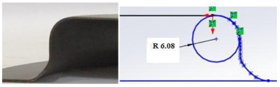
2 indicated that radius of convex and concave curve have dramatical influence on forming process. Due to high possibility of fitting with convex area, radii at die top and other convex areas (if any) inside can be easily formed and reach expected values. The study also showed that it is more difficult for material to fit with concave cure than convex curve in hydrostatic forming (
Fig. 1).
Fig. 1 Curve radii at die bottom
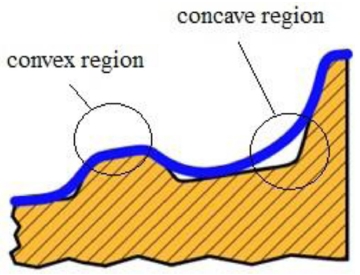
The difficulty in fitting with concave curve was also presented by D. Koller and S. Ulbrich.
3 In order to achieve smallest radius at cylinder bottom by hydrostatic forming, the authors used Abaqus to optimize the control of blank holder pressure and forming pressure. This method can be applied to enhance the efficiency of experiments.
However, a specific extend to which curve radius at die bottom depends on input parameters has not been evaluated. This causes trouble in defining input parameters, including technological parameters, die profile and initial shape of workpiece for designing any product with curve radius at the bottom.
Therefore, a process of forming a cylindrical product was researched to investigate the extent to which technological parameters and geometry parameters of die influence forming concave curve radius in hydrostatic forming.
In this paper, orthogonal second order design is employed to evaluate reliably the influence. The empirical planning is implemented for 3 variables: blank holder pressure, relative depth of die, relative thickness of product. Results are illustrated in functions and graphs, allowing the evaluation of each parameters. The results also enable us to select suitable input parameters for each type of product with each expected bottom radius.
2. Experiments
2.1 Research Method
Object: how the forming curve radius at the bottom of a cylindrical product with radius of Rd depends on input parameters.
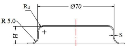
The selected product is shown in
Fig. 2. Radius region Rd is the typical concave area of the die.
Fig. 2The selected product

Research method: Combination of experimental research and numerical simulation has recently been one of the most widely used method for accurate results. In this research, simulation is done to define ranges of values to be investigated. After that, experiments are implemented to evaluate particular effects of given parameters. The paper focuses on experimental studies based on ranges of values of parameters that was defined by simulation before.
Orthogonal second order design is employed to solve the given problems because it permits influence of each parameter on product quality to be estimated in detail with high accuracy.
Objective function is Rd, curve radius at die bottom, because formation of this curve radius is considered one determinant of profile and quality of product.
Variables to be investigated:
- Blank holder pressure Qch: Together with forming pressure, blank holder pressure is a technological parameter that needs studying. This parameter allows hydrostatic forming process to take place, and it has big impact on the achievement of expected profile. The chosen range of value of blank holder pressure is Qch = (80-115) bar.
- Relative depth of die H*: Is defines as the ratio of die depth (H) and die diameter (d). Deep forming is not permitted in this technology, and the sheet cannot fit well with die profile due to initial free deformation. Therefore, it is proposed that different dies with different depths be created to facilitate forming process.
- Relative thickness of product
S*: Is defines as the ratio between the absolute thickness of workpiece (
S) and its diameter (
D0). This parameter influences heavily formation of cylinder bottom and thinning process on cylinder body. Values of
S* are given in
Table 2.
Other parameters such as friction coefficient, rate of deforming, material thickness, etc are considered to be constant.
Experimental results aim to evaluate the degree where the parameters above affect the formation of the curve radius at die bottom as functions and graphs, enabling the selection of an optimal set of parameters in order to obtain suitable curve radius.
2.2. Experiment Establishment
The selection is presented in detail as
Fig. 2. The chosen type of material is DC04 with mechanical, physical and chemical properties given in
Table 1. This material has been widely used in sheet forming.
Table 1Properties of DC04 steel
Table 1
|
Label |
Properties |
Equivalent label |
|
DC04 |
σm
(MPa) |
σf
(MPa) |
δ
(%) |
ρ
(kg/cm3) |
Russia-GOST
08kp Japan-JIS
SPCE |
|
314-412 |
210-280 |
38 |
7.8*10-3
|
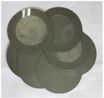
Geometry parameters of workpiece and die are provided in
Table 2. The workpieces were machined by wire electrical discharge machining to ensure the diameter
D0 = 110 mm (
Fig. 3).
Table 2Geometry parameters of workpiece and die
Table 2
|
Workpiece |
Die |
|
Diameter D0, mm |
110.0 |
Diameter d, mm |
70.0 |
|
Thickness S, mm |
0.8, 1.0, 1.2 |
Depth H, mm |
16.0, 18.0, 20.0 |
Relative thickness
S* (%)
S*=SD0
|
0.73, 0.91, 1.09 |
Relative depth
H* (%)
H*=Hd
|
23, 26, 29 |
Fig. 3Workpieces

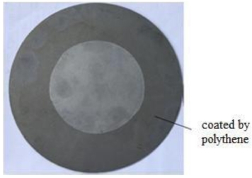
The workpiece’s flange was coated with one layer of polythene in order to avoid contact between workpiece and die surfaces (
Fig. 4). With friction coefficient
μ = 0.2, this layer allows the workpiece to slide easily and to be drawn into the die.
Fig. 4Workpiece coated with polythene
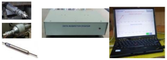
2.3 Experiment Devices
The experiment system is composed of 4 modules:
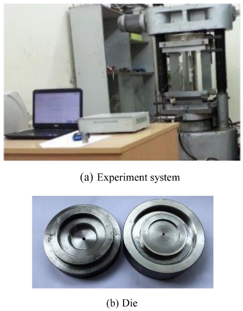
- 125-ton hydraulic press: is used to mount the die and create blank holder force (
Fig. 6)
- Hydrostatic die: is used to shape the workpiece
- High-pressure pump: is used to generate high-pressure liquid to form the workpiece
- Pressure and stroke measuring system is connected to computer (
Fig. 7)
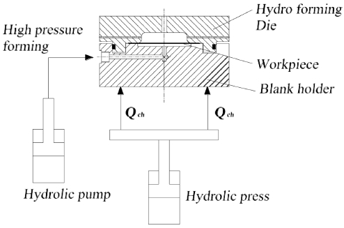
Fig. 5Schematic diagram of experiment system

Fig. 6Devices (a) and die (b)

Fig. 7Pressure-stroke meters
The die is fixed on the hydraulic press, and connected to the high-pressure pump and measuring system.
The workpiece is fixed between the blank holder and the die by blank holder force from the press.
High-pressure is pumped into the groove increasingly to form the product. The product is shaped according to the groove shape. Changes of pressure in grove, in cylinder and forming depth are collected by the measuring system and displayed on the computer screen.
Experiments were implemented on 125-ton hydraulic press.
Pressure measuring system was connected to a computer to supervise and adjust correctly required parameters (
Fig. 7).
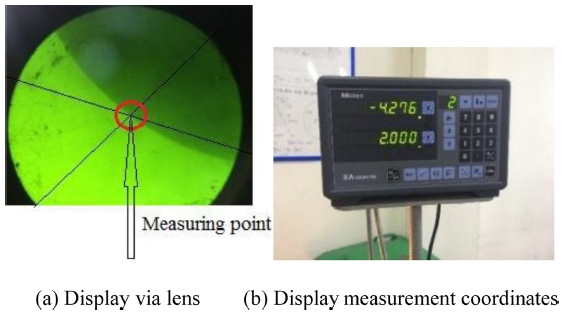
The measurement of product radius was deployed with optical meter μM21. The product was clamped on the machine (
Fig. 8), then rays of light were transferred through lens to project on the product profile (
Fig. 9(a)). The measurement coordinates are displayed as shown in
Fig. 9(b). Coordinates then were taken out and loaded into Solidworks software. After that, the most suitable value of radius was computed (
Fig. 10).
Fig. 8Optical meter μM21
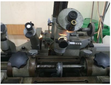
Fig. 9Coordinates of product profile displayed through lens and display screen

Fig. 10Establishment of product profile in Solidworks
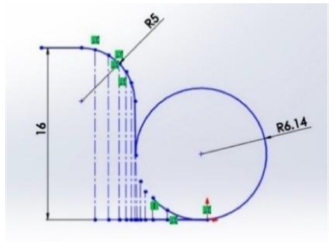
For each specimen, measure about 40 points to rebuild its profile as shown in
Fig. 11.
Fig. 11Measure curve radius Rd
2.4. Experiment Results
The orthogonal second order design for 3 variables requires 15 experiments, including 8 standard experiments, 1 in-center experiment, and 6 extension experiments as shown in
Table 4. In extension experiments, the input variables have extra values due to the variation in the expansion area. The results are as follows the
Table 3:
Table 3Input variables and survey values
Table 3
Input
variable |
Converted
variable |
Survey
value |
(+) |
(0) |
(−) |
(+α) |
(−α) |
|
Qch
|
x1
|
76,
80,
97.5,
115,
119
(bar) |
115 |
97.5 |
80 |
119 |
76 |
|
H*
|
x2
|
22,
23,
26,
29,
30
(%) |
23 |
26 |
29 |
30 |
22 |
|
S*
|
x3
|
0.7,
0.73,
0.91,
1.09,
1.12
(%) |
0.73 |
0.91 |
1.09 |
0.7 |
1.12 |
Table 4Values of input variables in 15 experiments
Table 4
|
N
0
|
Qch
|
H* |
S* |
|
1 |
+ |
- |
- |
|
2 |
+ |
+ |
- |
|
3 |
+ |
- |
+ |
|
4 |
+ |
+ |
+ |
|
5 |
- |
- |
+ |
|
6 |
- |
+ |
+ |
|
7 |
- |
- |
- |
|
8 |
- |
+ |
- |
|
9 |
0 |
0 |
0 |
|
10 |
+α
|
0 |
0 |
|
11 |
−α
|
0 |
0 |
|
12 |
0 |
+α
|
0 |
|
13 |
0 |
−α
|
0 |
|
14 |
0 |
0 |
+α
|
|
15 |
0 |
0 |
−α
|
Where:
(+): The upper level in the basic experiment
(0): Middle level in basic experiment
(−): Lower level in basic experiment
(+α): The upper level in extended area
(−α): Lower level in extended area
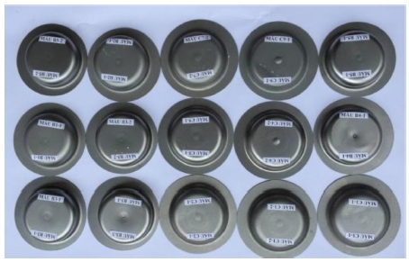
Fig. 12Experimental products

Curve radius at product bottom Rd in each specimens is demonstrated in
Table 5.
Table 5Experiment results
Table 5
|
No |
Rd (mm) |
|
1 |
6.31 |
|
2 |
6.35 |
|
3 |
6.36 |
|
4 |
6.84 |
|
5 |
10.2 |
|
6 |
8.49 |
|
7 |
7.60 |
|
8 |
7.59 |
3. Discussions
According to orthogonal second order design, the regression equation for Rd based on converted variable can be defined
Eqs. (2)-
(5):
where coefficients
bi,
b'i are given in
Table 6. Where coefficients
bj is calculated as follow
Eqs. (2)-
(5):
Table 6 Coefficients of regression equation
Table 6
|
Symbol |
Value |
|
b0
|
7.98 |
|
b1
|
-0.39 |
|
b2
|
0.43 |
|
b3
|
1.60 |
|
b12
|
-0.02 |
|
b13
|
-0.57 |
|
b23
|
0.26 |
|
b'1
|
0.42 |
|
b'2
|
0.19 |
|
b'3
|
0.31 |
In order to verify the coefficients, regeneration variance can be computed
Eqs. (7)-
(10):
Variance of coefficients in regression equation is defined and compared with Students standard, causing b12 to be omitted.
Residual variance is calculated to verify the suitability of the function:
Then, function test coefficient is:
Compared with Fischer standard Fα(f1, f2) with α = 0.05 and
Looking up the table, we have Fischer Fα(9. 2) = 19.4 > 11.3, so the regression function is satisfactory.
The relationship between Rd and converted variables can be written as:
Transferring into real variables,
Eq. (11) can be presented as:
In order to evaluate effect of each variable, considering boundary neighborhood of tested area, 3 equations can be inferred:
It can be inferred from coefficients in
Eqs. (13)-
(15) that the curve radius
Rd depends on
x3 (relative thickness of workpiece) at highest extent, and the extent decreases with respect to
x2 (relative depth of die) and
x1 (blank holder pressure) alternatively.
With respect to each value of blank holder pressure
Qch: Graphs were established from
Eq. (12) using Matlab, from that maximum and minimum curve radius Rd can be figured out.
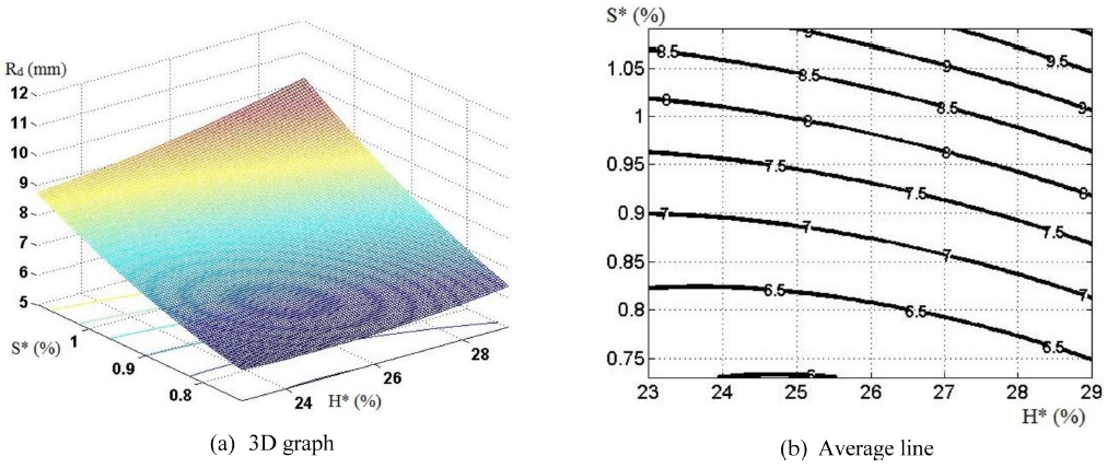
· Blank holder pressure Qch is set to be constant: When
Qch = 80 bar: minimum curve radius
Rdmin = 6.23 mm and maximum curve radius Rdmax = 11.5 mm (
Fig. 13)
Fig. 13 Dependence of Rd on H* and S* when Qch = 80 bar
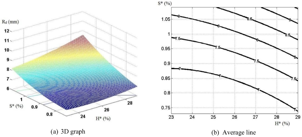
When
Qch = 97.5 bar:
Rdmin = 5.98 mm and
Rdmax = 10.1 mm (
Fig. 14);
Fig. 14 Dependence of Rd on H* and S* when Qch = 97.5 bar

When
Qch= 115 bar:
Rdmin = 6.58 mm and
Rdmax = 9.5 mm (
Fig. 15);
Fig. 15 Dependence of Rd on H* and S* when Qch = 115 bar

It can be seen from
Figs. 13-
15 that curve radius Rd reduces together with the decrease in relative thickness of workpiece
S* and relative depth of die
H*. In particular, the graph has a large angle of slope towards the axis of
S*, indicating that the formation of curve radius
Rd has great influence on the initial relative thickness of workpiece.
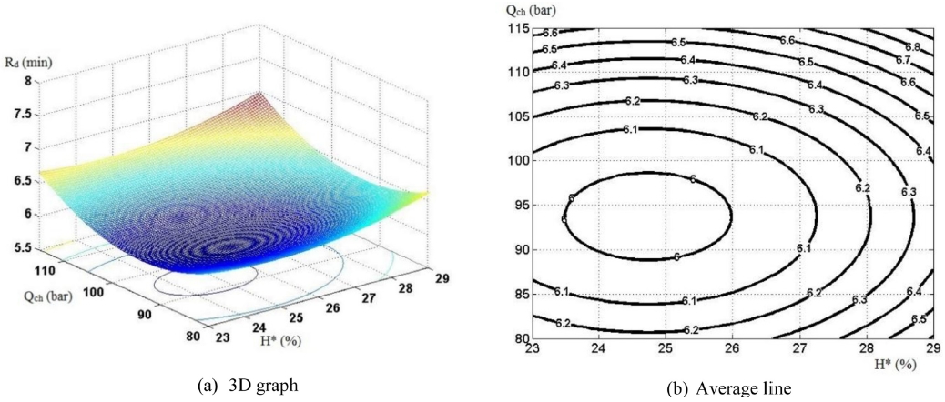
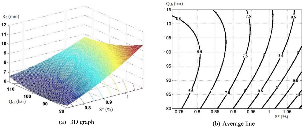
· With respect to each value of relative thickness of workpiece S*:
When
S* = 0.73 (%):
Rdmin = 5.97 mm and
Rdmax = 6.97 mm (
Fig. 16);
Fig. 16 Dependence of Rd on H* and Qch when S* = 0.73(%)
When
S* = 0.91 (%):
Rdmin = 6.99 mm and
Rdmax = 8.73 mm (
Fig. 17)
Fig. 17 Dependence of Rd on H* and Qch when S* = 0.91 (%)

When
S* = 1.09 (%):
Rdmin = 8.19 mm and
Rdmax = 11.47 mm (
Fig. 18);
Fig. 18 Dependence of Rd on H* and Qch when S* = 1.02 (%)
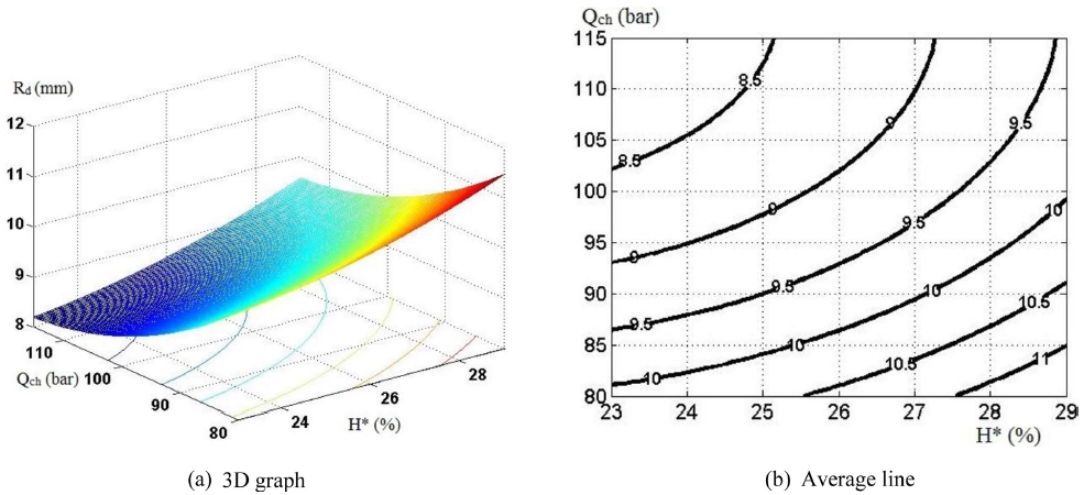
It can be observed from
Figs. 17 and
18 that there is a covariance in dependence of
Rd on
H*, that is, when
H* grows,
Rd increase and vice versa.
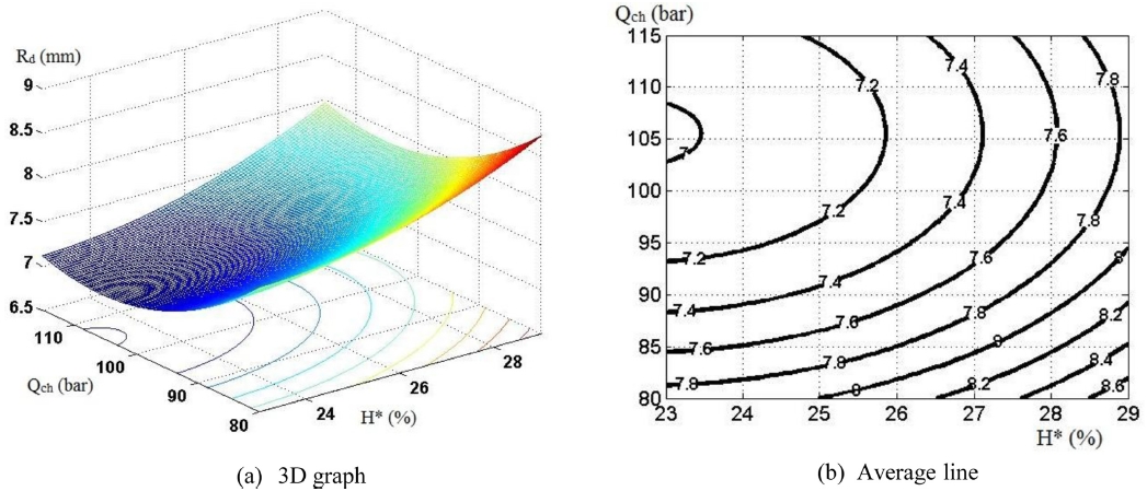
Fig. 16(b) shows that there exists an
H* value in the survey zone to achieve the minimum Rd radius. Therefore, with the relative thickness of workpiece greater than a defined value, the dependence of
Rd on
H* is shown to be simpler. Graphs in
Figs. 16-
18 also show that with respect to
Qch, Rd has a decrease when
Qch reaches a specific value, but Rd bounces up when
Qch continues increasing. As a result, there always exists one suitable value of
Qch so that
Rd can get minimum value.
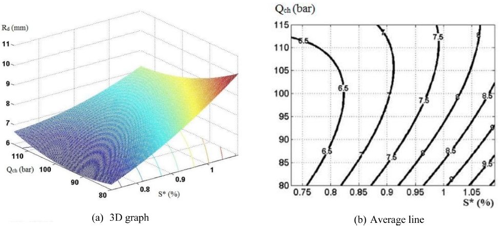
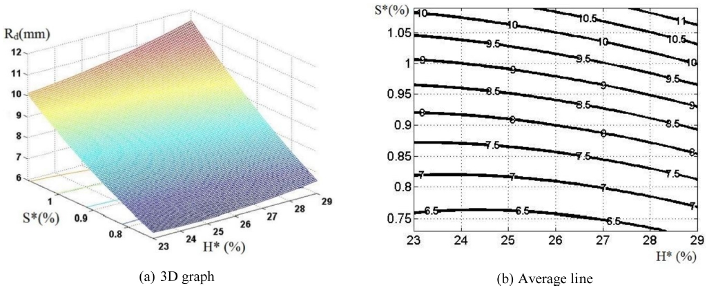
· With respect to each value of relative depth of die H*:
When
H* = 23 (%):
Rdmin = 6.03 mm and
Rdmax = 10.1 mm (
Fig. 19);
Fig. 19 Dependence of Rd on S* and Qch when H* = 23(%)

When
H* = 26(%):
Rdmin = 6.0 mm and
Rdmax = 10.6 mm (
Fig. 20);
Fig. 20 Dependence of Rd on S* and Qch when H* = 26 (%)
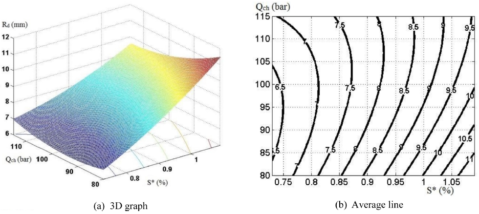
When
H* = 29 (%):
Rdmin = 6.35 mm and
Rdmax = 11.4 mm (
Fig. 21);
Fig. 21 Dependence of Rd on S* and Qch when H* = 29(%)

It can be noted from
Figs. 19-
21 that
Rd have dependence on
Qch and
S*. The case where
Rd depends on
Qch shows a similarity to
Fig. 16, which means that there always exists one suitable value of
Qch so that
Rd can get minimum value.
The situation above can be reasoned that:
- Beginning period: that blank holder pressure Qch increases makes curve radius Rd decrease. Because the growing blank holder pressure avoids the workpiece from instability on flange and assists in drawing material into the die. Moreover, together with blank holder pressure, forming pressure also rises theoretically, enabling the workpiece to be more easily pressed onto bottom area of the die. Therefore, the curve radius Rd will decrease and get the minimum value when Qch reaches a suitable value.
- Later period: after Rd gets the minimum value Rdmin, if Qch continues growing, the curve radius Rd bounces back. This can be argued that the increasing blank holder pressure makes it difficult for the material to be drawn into the die, preventing the workpiece from being pressed onto the die, especially the curve area. Consequently, the curve radius Rd increase in this period.
Furthermore, graphs in
Figs. 19-
21 also show that when the relative thickness of workpiece
S* increases, the curve radius Rd has the same tendency. This relationship has a good agreement with results in different cases above.
Hence, by experimental investigation, the formation of curve radius depends on following parameters:
-
Rd depends on all of 3 parameters (
Qch,
H*,
S*), where the relative thickness of workpiece
S* demonstrates the heaviest influence. The relationship is formulated in
Eq. (12).
- The curve radius Rd decreases more when the relative thickness of workpiece is smaller, the relative depth of die and the blank holder pressure reach a suitable value.
4. Conclusions
The experimental study indicates that the formation of curve radius at product bottom depends on all input parameters including blank holder pressure, relative depth of die, relative thickness of workpiece. In particular, in order for curve radius at product bottom to be smaller, the relative thickness of workpiece needs to be smaller, the relative depth of die and the blank holder pressure reach a suitable value.
The results have a great significance in designing thin-wall products, allowing easy selection and preventing damage or dimension deviation during manufacturing process.
In addition to curve radius at product bottom, other elements affecting product quality such as rate of thinning, thinning distribution, conicity, inverse elasticity, etc also needs paying attention to.
The achieved study opens the way for applying and deploying hydro static forming for sheet metal into thin wall manufacturing.
ACKNOWLEDGMENTS
This paper was presented at PRESM 2019
REFERENCES
- 1.
Kocańda, A. and Sadłowska, H., “Automotive Component Development by Means of Hydroforming,” Archives of Civil and Mechanical Engineering, Vol. 8, No. 3, pp. 55-72, 2008.
10.1016/S1644-9665(12)60163-0
- 2.
Sato, M. and Tomizawa, A., “Development of Double Sheet Hydroforming Technology,” Proc. of the International Automotive Body Congress 2010 Global Powertrain Congress 2010
- 3.
- 4.
Biography
- Nguyen Thi Thu
Doctor of Philosophy in Department of Metal Forming, School of Mechanical Engineering, Hanoi University of Science and Technology, Hanoi, Vietnam. Her favorite research includes special forming technologies and micro forming. In addition, she also gives lectures on sheet metal forming for 3rd and 4th year students at the university.
Tel: +84 976 512 385
- Nguyen Dac Trung
Associate Professor in the Department of Metal Forming, School of Mechanical Engineering, Ha-noi University of Science and Technology, Vietnam. He got Ph.D Degree at Technische Universität Dresden in 2003. His favourite research includes sheet forming, bulk forming and micro forming.
Tel: +84 913 059 227