ABSTRACT
The literature states that the existing guidelines mainly focus on the ultimate strength of uniform corroded joints in the Jacket-type re-assessment. However, joints are non-uniformly corroded in different shapes in reality. Results derived from theoretical equations in these scenarios are significantly different from the actual capacity of the frame joints. This paper studies the influences of thickness and corroded area on the T- joint’s ultimate strength for a chord based on the numerical model ABAQUS. Numerical results show the effects of location and dimension at corroded areas on the tubular joint ultimate strength. Moreover, this research proposes a new formula based on API to estimate the strength of T-joints connected with non-uniform corroded compressive braces in certain conditions. This equation is validated by comparison of the numerical simulation in independent cases.
-
KEYWORDS: Non-uniform corrosion, Tubular T-joint, Compression, Ultimate strength, Numerical models, ABAQUS program
1. Introduction
Tubular joints of Jacket steel structures are vital to determine the overall load-bearing capacity. Therefore, existing guidelines strictly regulate quality processes in a broad range of design, fabrication, supervision, and maintenance of these joints.
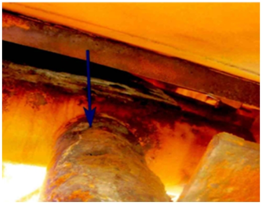
One of the most important effects on joint strength for a long time is the corrosion phenomenon. Although the steel fixed platforms are designed with corrosion protections like coating or sacrificial anode-derived cathodic protection etc., the joints are located at the intersection between pipes. Consequently, it is difficult to protect or maintain them periodically, compared with other positions. Furthermore, platforms exploiting in Vietnam Sea are corroded more seriously and complicatedly than expected (
Figs. 1 to
3). In some projects, designed corrosion thickness ranges between 0.2 mm to 0.3 mm per year. Meanwhile, according to surveys of wellhead platforms in the White Tiger field, the average corrosion thickness is able to reach roughly 0.45 mm per year at some platforms
[1]. The thickness difference at locations in the same section can vary more than two times. Consequently, the simulation of tubular joints meets difficulties and then considers incorrect when estimating strength checks based on standardderived formulae compared with actual cases.
Fig. 1 Platform BK-1 at White Tiger field was corroded (photo by VSP)
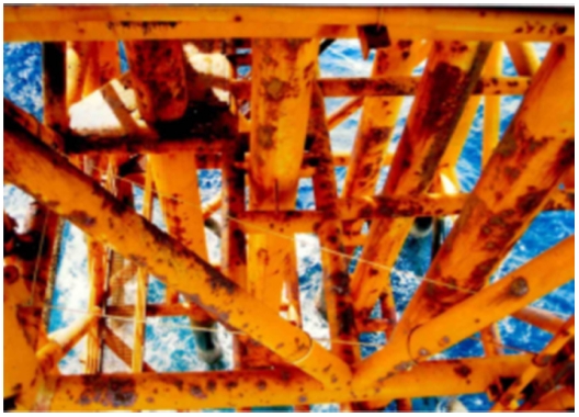
Fig. 2 A tubular joint in the platform MSP6 at White Tiger field was corroded (photo by VSP)
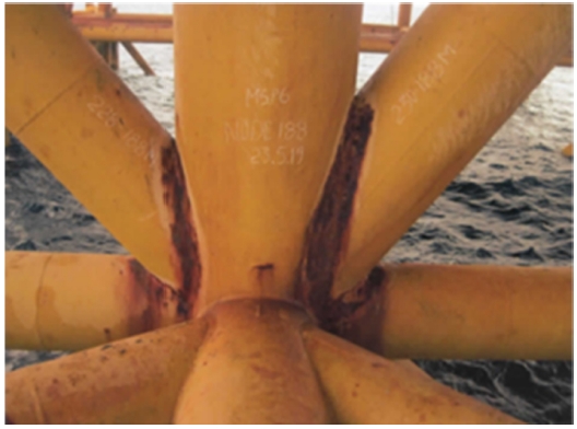
Fig. 3 A tubular joint in the platform MSP6 was corroded (photo by VSP)
Investigations into the physical mechanism of strength checks, the tubular joint is destroyed at positions when the von Mises stress at the brace/chord intersection is greater than the material strength. The von Mises stress is caused by the chord and brace's internal forces. For simplicity, guideline API RP 2A
[2] assumes that the internal force originating from the braces is an effect on the tubular joints, while the force on the chords is a factor that affects the strength. Accordingly, the strength of tubular joints depends on the material, the chord’s thickness, the types of chord, and the internal forces of the chord.
However, being non-uniform corrosion, the thickness and shape of the chord section are changed. Actually, the formulae of strength for corroded pipe are not yet fully developed in the standard API so far.
There are various published studies worldwide related to the checks of tubular joint strength. However, OTH
[3], Azari-Dodaran and Ahmadi
[4], and Mia et al.
[5] focused mainly on joint strength checks of different tubular joints; Moffat et al.
[6], and Van der Vegte and Makino
[7] investigated the influences of geometric forms and boundary conditions on tubular strength; Nassiraei et al.
[8], P.S. Prashob et al.
[9], Murugan et al.
[10], and Shubin et al.
[11] estimated the strengthening joints; Jalal and Bousshine
[12], Moya
[13], Stransky
[14] concentrated on joint strength checks by numerical models.
The above research mentioned various problems, containing the influential scope of punching forces, the influences of boundary conditions at joints, internal forces of chords and braces, the stress distribution and damaged shape of the chord section at tubular joints, the impact of strengthening patterns on joint strength, the validate of numerical and physical models, etc. Some results will be used and validated in this research.
The research on the strength of corroded joints is mainly focused on uniform corrosion over the whole section or pitting form and their application on strengthened joints. The strength of uniform corroded CFRP-strengthened T-joints on a segment of pipe was investigated by Mohamed et al.
[15]. Zuo et al.
[16] researched the behaviour of corroded T-joints using strengthening by CFRP and grouting.
Especially, Mohamed et al.
[15] proposed a new equation to include the effect of the corrosion phenomenon by using the power function of the ratio between the corroded chord thickness and the intact thickness pre-corrosion.
Nevertheless, previous studies have not yet focused on the effects of the chord’s corrosion position on tubular strength and the effect of the corrosion area on this strength.
The objective of this paper is to deal with the two above problems. However, this research only concentrates on T-joints associated with compression braces. Furthermore, the paper investigates the tubular strength of the chord’s diameter and thickness in different scenarios using ABAQUS. Accordingly, the influential scope of the corrosion area and additional factors will be built up to modify the strength formulae in API for corroded T-joints under compression. The details will be given in the following sections.
2. Methods
2.1 Build-up Model of the Tubular Joints for Strength Checks
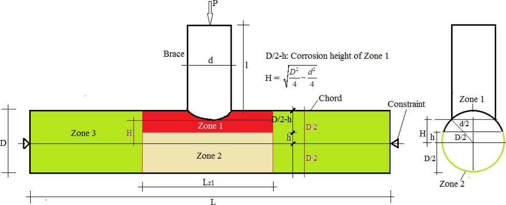
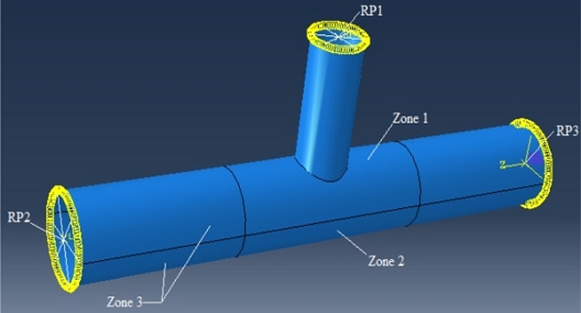
Considering a T-joint as described in
Fig. 4, the corresponding outer diameter and thickness of the brace are
d and
t, respectively. These parameters of the chord are
D and
T, respectively. The brace is subjected to an axial compression force
P. The lengths of the brace and chord are
l and
L, respectively. The corrosion data are applied in every region from Zone 1 to Zone 3. Where
D⁄2 –
h denotes the corroded area height at Zone 1, and
h is the distance from the tubular centre to the edge of Zone 1.
Fig. 4A sketch of a corroded tubular T-joint
The length
l is chosen to be short enough to keep stable of the brace. The length
L is long enough not to have effects on the stress distribution at the brace/chord intersection. According to Moffat et al.
[6], the length
L should satisfy the ratio
L⁄
D ≥ 6. The force
P satisfies the compressive strength of the brace and the bending strength of the chord. The two end connections are considered pinned joints since the actual chord has a rotation angle. The effect of the chord’s axial force on tubular strength is ignored in this research.
The model is divided into three types depending on their objectives.
- Type 1: the joint model is intact, applying to validate the suitability of the numerical model and API-based calculations. The parameters of database id. from c-01 to c-09 are given in
Table 1.
Table 1Parameters of intact joints
Table 1
Database
id. |
Chord section
D × T [mm] |
L
[m] |
Brace section
d × t [mm] |
l
[m] |
|
c-01 |
813 × 25 |
5 |
508 × 16 |
2 |
|
c-02 |
813 × 20 |
5 |
508 × 16 |
2 |
|
c-03 |
813 × 15 |
5 |
508 × 16 |
2 |
|
c-04 |
1,020 × 30 |
6.5 |
610 × 16 |
2 |
|
c-05 |
1,020 × 25 |
6.5 |
610 × 16 |
2 |
|
c-06 |
1,020 × 20 |
6.5 |
610 × 16 |
2 |
|
c-07 |
1,270 × 30 |
8 |
813 × 19 |
2 |
|
c-08 |
1,270 × 25 |
8 |
813 × 19 |
2 |
|
c-09 |
1,270 × 20 |
8 |
813 × 19 |
2 |
- Type 2: Modeling is used to assess the influence of corroded location on joint strength. As mentioned in
Figure 4, this paper considers only the effect of tubular thickness variation in 3 zones on the joint strength. Parameter data of corroded joints in each zone are shown in
Table 2, and more details are shown in
A1.1 Appendix.
Table 2Parameter data of corroded joints in each section
Table 2
Database
id. |
Chord section
D × T [mm] |
L
[m] |
Brace section
d × t [mm] |
l
[m] |
|
c-10 |
813 × 25 |
5 |
508 × 16 |
2 |
|
c-11 |
1,020 × 30 |
6.5 |
610 × 16 |
2 |
|
c-12 |
1,270 × 30 |
8 |
813 × 19 |
2 |
|
c-13 |
813 × 25 |
5 |
508 × 16 |
2 |
|
c-14 |
813 × 25 |
5 |
508 × 16 |
2 |
|
c-15 |
1,020 × 30 |
6.5 |
610 × 16 |
2 |
|
c-16 |
1,020 × 30 |
6.5 |
610 × 16 |
2 |
|
c-17 |
1,270 × 30 |
8 |
813 × 19 |
2 |
|
c-18 |
1,270 × 30 |
8 |
813 × 19 |
2 |
- Type 3: Modeling is applied to assess the effect of the corrosion area on joint strength for Zone 1. Based on
Figure 4, the corroded area scale of Zone 1 is measured by parameters
Lz1 and 0.5
D-
h Data on the tubular joint model is provided in
Table 3, and more details are shown in
A1.2 Appendix.
Table 3Parameter data of corroded joints in Zone 1
Table 3
Database
id. |
Chord section
D × T [mm] |
L
[m] |
Brace section
d × t [mm] |
l
[m] |
|
c-19 |
813 × 25 |
5 |
508 × 16 |
2 |
|
c-20 |
813 × 25 |
5 |
508 × 16 |
2 |
|
c-21 |
813 × 25 |
5 |
508 × 16 |
2 |
|
c-22 |
813 × 25 |
5 |
508 × 16 |
2 |
|
c-23 |
1,020 × 30 |
6.5 |
610 × 16 |
2 |
|
c-24 |
1,020 × 30 |
6.5 |
610 × 16 |
2 |
|
c-25 |
1,020 × 30 |
6.5 |
610 × 16 |
2 |
|
c-26 |
1,020 × 30 |
6.5 |
610 × 16 |
2 |
|
c-27 |
1,270 × 30 |
8.0 |
813 × 19 |
2 |
|
c-28 |
1,270 × 30 |
8.0 |
813 × 19 |
2 |
|
c-29 |
1,270 × 30 |
8.0 |
813 × 19 |
2 |
|
c-30 |
1,270 × 30 |
8.0 |
813 × 19 |
2 |
The model results based on type 3 are used to establish a formula to check the corroded T-joint strength.
2.2 Strength Analysis of T-joints under Brace Axial Compression in API
2.2.1 Strength of Non-corrosion Tubular Joints
The allowable compression force
Pa of a T-joint under brace axial compression can determine as
equation (1)
Where Fyc is the yield limit of the material; T is the chord thickness; θ is the angle between the chord and brace, for the T-joint; θ = 90o; FS is the safety factor, so FS = 1.6 means the joint works in the elastic phase. However, this paper only researches tubular joint checks based on ultimate strength, so FS = 1 and Pa is ultimate compression force.
Qu is the strength factor, dependent on the joint type and the status of the bearing load. For T-joints, if the brace is compressive, then
Qu can estimate as
equation (2).
Where β = d/D is the brace to chord diameter ratio. Qf is the factor, dependent on chord internal force, if FS = 1, Qf can determine as below:
Where Pc,Mipb,Mopb are the axial force, in-plane and out-plane bending moment, respectively, and Mc is the total moment of the chord.
Py is the ultimate axial capacity of the chord, corresponding to the yield stress. Mp is the plastic moment capacity of the chord.
For T-joints associated with a compression brace, coefficients C1 = 0.3, C2 = 0 and C3 = 0.8.
2.2.2 Ultimate Strength of Non-uniform Corroded Joints
As mentioned above, there has not been any research proposing formulae to assess the strength of non-uniform corroded joints. In general cases, von Mises should be analyzed. The ultimate strength problem happens when the von Mises stress reaches to yield limit of the material. Therefore, the most effective approach is to analyze based on the numerical model to solve this matter. The numerical method will describe in the following section. This part will provide some matters as followings:
For T-joints mentioned in
Figure 4, if the brace is subjected to a compressive force, the chord section exerts shear stress and bearing moment-caused stress.
When fully plastic happens at a section, the shear stress at the brace/chord intersection mainly relies on a square of the chord thickness at that position, and the bending moment–exerted stress depends on the plastic moment capacity of the tubular section.
The larger corroded area around the brace/chord intersection makes the less strength capacity of the chord. The strength capacity will be reduced to the value of an intact joint in which its chord thickness equals the corroded thickness.
The brace thickness causes only shear stress increase and has an insignificant influence on the strength of tubular joints. Therefore, the corrosion on the chord only is investigated in this paper.
2.3 Numerical Simulation of Stress Checks on Corroded T-joints
The tubular joints are simulated by ABAQUS (Dassault Systèmes Simulia Corp
[17]). Some main matters are provided as follows:
- Tubular joints are modeled based on geometric data mentioned in
Section 2.1. In empirical equations of the joint strength, the effect of weld geometry is insignificant then can be ignored. In order to change the thickness and decrease the amount of computation in the model, joints are simulated by shell elements.
- Reference points
RP2 and
RP3 are created at two ends of the chord, corresponding to the working of 2 relevant sections to impose boundary conditions and internal forces of the chord. The point
RP1 is put at the brace’s end to apply the compression force (
Figure 5) and to obtain displacement results.
Fig. 5A tubular T-joint model
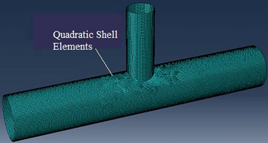
- Pipes have meshed into quadrilateral elements with four-node S4R. The size of elements is properly chosen to make the stress at the brace/chord intersection convergent (
Figure 6). The influence of element meshes on the tubular strength is not the objective of this study. Some meshes are selected to use in this model, as described in
Figures 5 and
6.
Fig. 6Tubular T-joint meshes
Results of the joint strength corresponding to element sizes of 3 cm, 4 cm, and 5 cm are given in
Table 4. Clearly, the 3-cm element size shows the convergence of the ultimate strength for tubular joints; therefore, this type of shell size will be applied to all calculations in this paper.
Table 4The effect of element sizes on the ultimate strength of tubular joints
Table 4
|
Database id. |
Element size
[cm] |
Pa in
ABAQUS
[MN] |
Pa (API)
[MN] |
Error [%] |
|
c-01 |
5 |
3.27 |
2.99 |
9.4 |
|
4 |
3.13 |
4.7 |
|
3 |
3.12 |
4.4 |
|
c-04 |
5 |
4.50 |
4.17 |
7.9 |
|
4 |
4.38 |
5.0 |
|
3 |
4.35 |
4.3 |
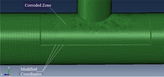
The corroded tubular pipe is divided into three zones to impose corrosion data, as mentioned in
Tables 2 and
3. Since the pipe is corroded, starting from outside to inside, it is necessary to adjust the coordinates of points corresponding to the chord based on the corrosion data.
At any one point on the chord with a diameter
D, and a corrosion thickness Δ
T, the new coordinates
xc,
yc satisfy
equations (8):
Where x, y are the pre-corrosion coordinates of xe, yc.
The corroded joint simulation is given in
Figure 7.
Fig. 7Modification of joint coordinates at corroded zones

After establishing a proper model, the Riks method is chosen (Dassault Systemes Simulia Corp
[17]) to analyze the tubular joint stress with taking non-linear effects into account; for more details, see Vu and Hà
[18].
3. Results
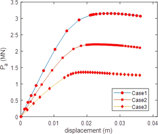
3.1 Validation of the Numerical Model
In this part, the ultimate strength of the intact tubular points is analyzed using data in the first nine cases (
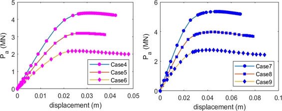
Table 1) in the ABAQUS model.
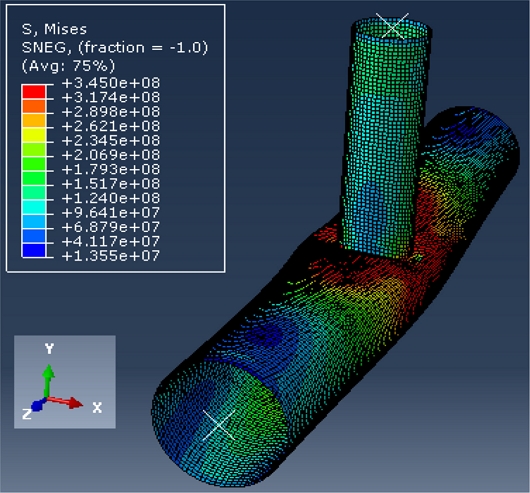
Figure 8 presents the relationship between axial forces and displacements at the force point RP1 in cases c-01 to c-03 (cases c-04 to c-09 see
A2.1.1 Appendix), and
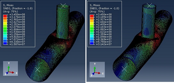
Fig. 9 illustrates collapsed states of the joints.
Fig. 8Ultimate compression force of T-joints in three first cases

Fig. 9Collapsed configurations of T-joints – case c-01

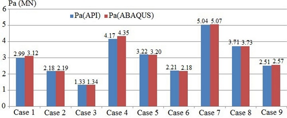
The ABAQUS-based results are comparable with the standard API values (
Figure 10). The greatest difference is roughly 4%. It proves a good agreement between the numerical method and formulae in the guideline. Next, the numerical model will be applied to determine the ultimate strength of the tubular joint for non-uniform corroded pipes and then to establish the new equation.
Fig. 10Ultimate compression force comparisons of T-joints based on API standard and numerical models

3.2 Ultimate Strength Assessment of Corrosion-impacted Regions for Tubular Joints
3.2.1 The Length at Zone 1 (Lz1)
According to the research of Mohamed et al.
[15], when
Lz1 >
D, the ultimate strength of tubular joints changes insignificantly compared with those at
Lz1 =
D. Moreover, Lesani et al.
[19] mentioned that the plastic area around joints lay in a range of length
Le=2×6DT. Therefore, this paper proposes this length L
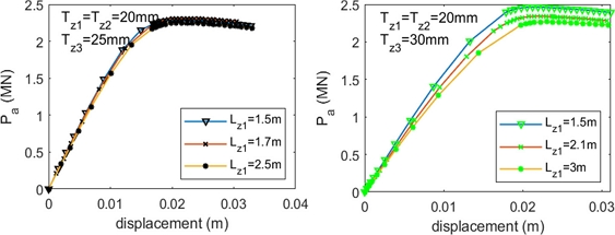
e as a limitation of a corroded area which has affected the ultimate strength of the joint. The numerical model is used to validate the suggestion, responding to the test id. from c-10 to c-12. The results are provided in
Table 5,
Figures 11 and
A2.3 Appendix
Table 5Ultimate compression force of uniform corrosion tubular T-joints at Zone 1
Table 5
Database
id. |
Tz1 = Tz2
[mm] |
Lz1
[m] |
Le
[m] |
Tz3
[mm] |
Lz3
[m] |
Pa
[MN] |
|
c-10 |
20 |
1.5 |
1.7 |
25 |
1.75 |
2.29 |
|
20 |
1.7 |
25 |
1.65 |
2.26 |
|
20 |
2.5 |
25 |
1.25 |
2.25 |
|
c-11 |
20 |
1.5 |
2.1 |
30 |
2.25 |
2.34 |
|
20 |
2.1 |
30 |
2.2 |
2.30 |
|
20 |
3.0 |
30 |
1.75 |
2.26 |
|
c-12 |
20 |
2 |
2.3 |
30 |
3 |
2.90 |
|
20 |
2.3 |
30 |
2.85 |
2.73 |
|
20 |
3 |
30 |
2.5 |
2.67 |
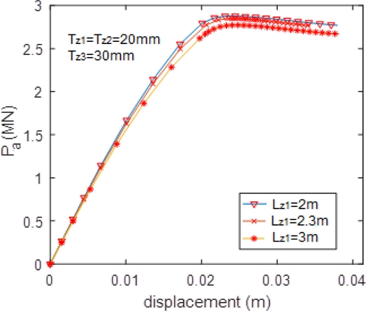
Fig. 11Ultimate force results of tubular T-joints case c-12

Based on the results, it can be seen that the formulae proposed by Lesani et al.
[19] are relatively well. When the length of the corrosion area is more than
Le, the ultimate strength of the corroded joints will slowly deviate and be convergent to the strength of an intact joint in which its thickness equals the corroded thickness (corresponding to cases c-03, c-06 and c-09 in
Figure 8). The most significant error is 6.2%.
3.2.2 Corrosion Effects at Zones 1 and 2
The changes in the ultimate strength of corroded tubular joints at Zones 1 and 2 are investigated. Their geometry data are given in
Table 2, and corrosion data corresponding to the cases from c-13 to c-18 are in
Appendix A1.1. The numerical results are shown in the following figures (
Figures 12 and
A2.4 Appendix).
Fig. 12Ultimate compression force results of tubular T-joints – cases c-13, c-14
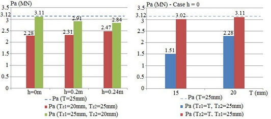
They indicate the corrosion effects in Zone 1 on tubular strength are pretty substantial. The change can vary by roughly 50%. Meanwhile, the corrosion in Zone 2 has a minor influence on the strength. The maximum value is roughly 10% when the corrosion perimeter in Zone 2 occupies more than 70% of the tubular perimeter. The corrosion increases in Zone 1 make the tubular joint strength quickly decrease up to 1.5 times, while the corrosion thickness increases in Zone 2, corresponding to a slight decrease, ranging from 2% to 3%.
It can explain that the tubular joint strength mainly relies on the chord’s surface area at the brace interaction, which is directly impacted by the chord. In Zone 2, the effect on stress distribution of all the chord sections is crucial, so it does not have any influence on the tubular joint strength. Consequently, the corrosion in Zone 2 is ignored in this research.
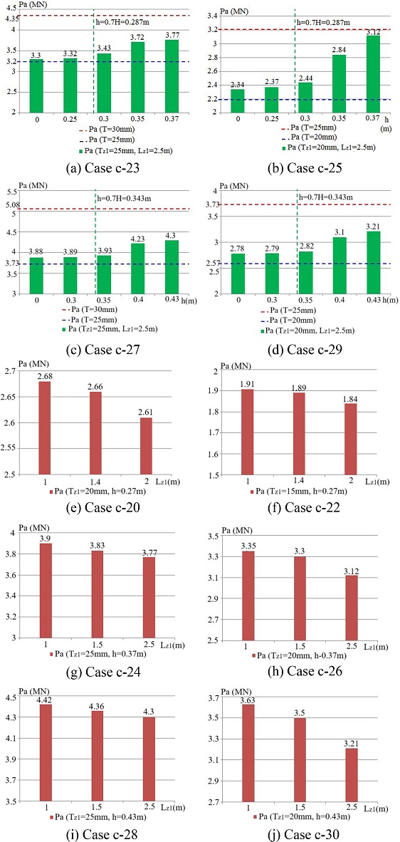
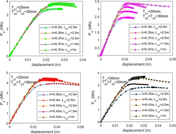
3.2.3 Effect of Corrosion Dimension at Zone 1
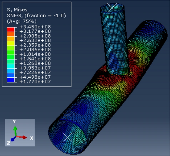
Fig. 13Ultimate compression force results of corroded tubular T-joint (chord 813 × 25 mm and brace 508 × 16 mm)
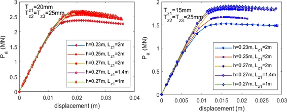
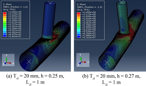
Fig. 14Collapsed configurations of corroded T-joints – chord 813 × 25 mm and brace 508 × 16 mm, Tz1 = 20 mm, h = 0.23 m, Lz1 = 1 m

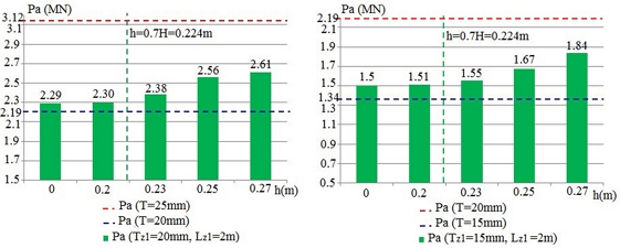
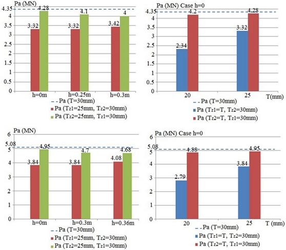
Fig. 15Ultimate compression force of tubular T-joints depending on h – cases c-19, c-21

Based on the analysis results, the effects of corroded factors on ultimate strength can be given as follows:
- Corroded thickness is a primary factor impacting the tubular joint ultimate strength. It can be explained that the joint strength capacity depends on the squared thickness of the chord at a joint intersection.
- The corrosion height significantly affects the tubular joint ultimate strength. In
Figure 4, the corrosion height at Zone 1 varies from elevation 0.5D-h to the chord top. According to the numerical results, two scenarios can be classified relying on the corrosion height. Scenario 1 occurs when
h≥0.7H=0.7D2/4-d2/4, if the corroded area height increases (
h reduces), the ultimate strength decreases. Conversely, when the corrosion height decreases, the ultimate strength of the corroded tube will gradually increase until it reaches the ultimate value of the intact joint. Cases c-19, c-21, c-23, c-25, c-27, and c-29 indicate that when the corroded area height increases, the maximum deduction rate of ultimate strength is more than 33% for the same corroded thickness. When h < 0.7H, the corroded tubular strength hardly changes compared with a uniform joint with chord thickness T
z1 in case 2.
- In the limitation of Lz1≤2×6DT, the corroded area length has a small impact on joint strength. When Lz1 increases the joint strength decreases slightly (only 13%) for the same corroded thickness.
- When corroded thickness increases, the influential scope of the corroded area on the tubular joint ultimate strength is more significant.
3.3 Build up a New Equation of the Corroded Tubular Strength
Considering
Tcc is the uniform thickness of the corrosion chord,
Pa(
Tcc) is the ultimate compression force of an intact tubular, corresponding to the thickness
T = (
Tcc). Based on
equation (1):
The tubular strength limits in a range of 0.7
H ≤
h ≤
H and
d≤Lz1≤2×6DT is denoted
Pac and connected to
Pa(
Tcc) in
equation (10):
Where the coefficient
δc is formulated dependent on
T,
Tcc,
h and
Lz1 based on the linear regression method (Vu
[20]):
The coefficient
a0,
a,
b was determined based on the least square method (Vu
[20]) in 30 tests corresponding to the 30 numerical model results, summarizing in
Table 6.
Table 6Ultimate compression force results of T-joints for regression analysis
Table 6
|
Case |
Tcc
[mm] |
h
[m] |
Lz1
[m] |
Pa (Tcc)
[MN] |
Pac
[MN] |
|
t-01 |
20 |
0.23 |
2 |
2.19 |
2.38 |
|
t-02 |
20 |
0.25 |
2 |
2.19 |
2.56 |
|
t-03 |
20 |
0.27 |
2 |
2.19 |
2.61 |
|
t-04 |
20 |
0.27 |
1.4 |
2.19 |
2.66 |
|
t-05 |
20 |
0.27 |
1 |
2.19 |
2.68 |
|
t-06 |
15 |
0.23 |
2 |
1.34 |
1.55 |
|
t-07 |
15 |
0.25 |
2 |
1.34 |
1.67 |
|
t-08 |
15 |
0.27 |
2 |
1.34 |
1.84 |
|
t-09 |
15 |
0.27 |
1.4 |
1.34 |
1.89 |
|
t-10 |
15 |
0.27 |
1 |
1.34 |
1.91 |
|
t-11 |
25 |
0.3 |
2.5 |
3.22 |
3.43 |
|
t-12 |
25 |
0.35 |
2.5 |
3.22 |
3.72 |
|
t-13 |
25 |
0.37 |
2.5 |
3.22 |
3.77 |
|
t-14 |
25 |
0.37 |
1.5 |
3.22 |
3.83 |
|
t-15 |
25 |
0.37 |
1 |
3.22 |
3.9 |
|
t-16 |
20 |
0.3 |
2.5 |
2.2 |
2.44 |
|
t-17 |
20 |
0.35 |
2.5 |
2.2 |
2.84 |
|
t-18 |
20 |
0.37 |
2.5 |
2.2 |
3.12 |
|
t-19 |
20 |
0.37 |
1.5 |
2.2 |
3.33 |
|
t-20 |
20 |
0.37 |
1 |
2.2 |
3.35 |
|
t-21 |
25 |
0.35 |
2.5 |
3.73 |
3.93 |
|
t-22 |
25 |
0.4 |
2.5 |
3.73 |
4.23 |
|
t-23 |
25 |
0.43 |
2.5 |
3.73 |
4.3 |
|
t-24 |
25 |
0.43 |
1.5 |
3.73 |
4.36 |
|
t-25 |
25 |
0.43 |
1 |
3.73 |
4.42 |
|
t-26 |
20 |
0.35 |
2.5 |
2.57 |
2.81 |
|
t-27 |
20 |
0.4 |
2.5 |
2.57 |
3.1 |
|
t-28 |
20 |
0.43 |
2.5 |
2.57 |
3.21 |
|
t-29 |
20 |
0.43 |
1.5 |
2.57 |
3.5 |
|
t-30 |
20 |
0.43 |
1 |
2.57 |
3.63 |
Considering
lndc=Y,lnao=c,lnTTcchH=X1,lnTTccLz112DT=X2, the
formula (11) can be rewritten as:
Letting Y-k is a set of data of Y corresponding to the 30 tests originated from the numerical model (t-01 to t-30). The sum of the random errors squared can be expressed as:
In order to minimize the error S, we have a matrix problem:
Factors a, b, and c can be found as the roots of the
equation (15). Consequently, results can be found:
a0 = 1.033,
a = 1.218 and
b = -0.497. After that, the coefficient
δc can be determined in
equation (11):
Finally, the above formula can be written as:
The coefficient can be gained as below:
The coefficient is approximately 1, so the proposed formula is acceptable.
3.4 Validation of the New Predictive Formula
A corroded tubular model is investigated with the input data below (
Table 7) to validate the
formula (16).
Table 7Corroded joint data for verification of the new formula
Table 7
|
Case |
Tcc
[mm] |
h
[m] |
Lz1
[m] |
|
v-01 |
25 |
0.3 |
2.5 |
|
v-02 |
25 |
0.3 |
1.2 |
|
v-03 |
20 |
0.3 |
2.5 |
|
v-04 |
20 |
0.3 |
1.2 |
The results of the tubular T-joint ultimate compression force based on the numerical model and the new empirical
formula (17) are shown in
Table 8. The maximum error is only 3%, meaning the new formula can be acceptable. On the other hand, when we consider the corrosion is non-uniform (
pac), the maximum difference of 33% can be seen compared with that in uniform corrosion (
Pa(
Tcc)). The difference depends on the dimension of the corrosion area.
Table 8Comparison of ultimate compression force results between the new formula and the numerical model
Table 8
|
Case |
Pa (Tcc)
[MN] |
δc |
Pac
[MN] |
Pac (ABAQUS)
[mm] |
Error
[%] |
|
v-01 |
5.03 |
1.118 |
5.63 |
5.71 |
1.5 |
|
v-02 |
5.03 |
1.176 |
5.92 |
5.88 |
0.6 |
|
v-03 |
3.51 |
1.232 |
4.33 |
4.4 |
1.7 |
|
v-04 |
3.51 |
1.378 |
4.84 |
4.69 |
3 |
4. Conclusions
According to the investigation of the strength of T-joints with the compression brace in the numerical model and theoretic formulae, conclusions can be made as follows.
The corrosion phenomenon influences the ultimate strength of T-joints in different scopes, depending on corroded position and dimension. Particularly the corrosion outside the area Le=2×6DT around the brace/chord intersection has a minor effect on the tubular strength. The corrosion of the below semitubular chords insignificantly impacts the tubular strength. When the corrosion in Zone 2 gradually develops until the corrosion occupies 0.7 times the tubular perimeter, the tubular strength is able to decrease moderately, relying on the corrosion thickness.
Corrosion in Zone 1 plays a crucial role in tubular strength determination. Apart from the corrosion thickness, the corrosion area has a significant influence. The corrosion height has a more substantial effect, and until it reaches the limitation of 0.3 H, the strength is convergent to the value, corresponding to a pipe that is corroded an upper semi-tubular. When the corrosion length changes into d ≤ Lz1 ≤ Le, the tubular strength can be impacted. When the corrosion height is relatively small, the effect of Lz1 can be seen.
Numerical models are proved to be quite effective. For the intact joints in
Table 1, the maximum error of ultimate compression force results between the numerical method and API standard is only about 4%. Moreover, for validated cases of the corroded joints in
section 3.4, the maximum error of the results between the numerical models and the new formula is only about 3%. In general cases, it is confirmed that complicated corrosion distributions can use the numerical model to investigate the tubular strength due to cost-effective expenses associated with trustworthy results. Note that the designed strength of the tubular joints can be determined by dividing ultimate strength by FS = 1.6 to ensure the tubular joint works in the elastic stage.
The formula proposed in this paper applies to the corrosion in Zone 1 where the influential scope of corrosion on the tubular joint ultimate strength is the most substantial. The formulae are validated in different numerical models. The match agreements between them prove the conformity of the equation. However, physical models should be carried out to validate the new equation before applying it in real projects.
The research helps surveyors, consultants and offshore platform owners give more appropriate responses for their structural safety in similar situations regarding the effects of corroded position and dimension on the tubular joint ultimate strength.
ACKNOWLEDGMENTS
The research described in this paper was financially supported by the Ministry of Education and Training in Scientific Project number B2021-XDA-04.
REFERENCES
- 1.
- 2.
- 3.
- 4.
Azari-Dodaran, N., Ahmadi, H., (2019), Static behavior of offshore two-planar tubular KT-joints under axial loading at fire-induced elevated temperatures, Journal of Ocean Engineering and Science, 4(4), 352-372.
10.1016/j.joes.2019.05.009
- 5.
Mia, M., Islam, M., Kabir, A., Islam, M., (2020), Numerical analysis of tubular XT joint of jacket type offshore structures under static loading, BMJ, 6(1), 299-318.
- 6.
Moffat, D., Kruzelecki, J., Blachut, J., (1996), The effects of chord length and boundary conditions on the static strength of a tubular T-joint under brace compression loading, Marine Structures, 9(10), 935-947.
10.1016/0951-8339(96)00007-X
- 7.
Van der Vegte, G., Makino, Y., (2010), Further research on chord length and boundary conditions of CHS T-and X-joints, Advanced Steel Construction, 6(3), 879-890.
10.18057/IJASC.2010.6.3.5
- 8.
Nassiraei, H., Lotfollahi-Yaghin, M. A., Ahmadi, H., (2016), Static strength of doubler plate reinforced tubular T/Y-joints subjected to brace compressive loading: Study of geometrical effects and parametric formulation, Thin-Walled Structures, 107, 231-247.
10.1016/j.tws.2016.06.009
- 9.
Prashob, P., Shashikala, A., Somasundaran, T., (2018), Effect of FRP parameters in strengthening the tubular joint for offshore structures, Ocean Systems Engineering, 8(4), 409-426.
- 10.
Murugan, N., Kaliveeran, V., Nagaraj, M., (2020), Effect of grooves on the static strength of tubular T joints of offshore jacket structures, Materials Today: Proceedings, 27, 2541-2545.
10.1016/j.matpr.2019.10.132
- 11.
Shubin, H., Yongbo, S., Hongyan, Z., (2013), Static strength of circular tubular T-joints with inner doubler plate reinforcement subjected to axial compression, The Open Ocean Engineering Journal, 6, 1-7.
10.2174/1874835X01306010001
- 12.
Jalal, S. E., Bousshine, L., Elastoplastic behaviour of T, Y, DT and DY-tubular joints under axial loading, IOSR Journal of Mechanical and Civil Engineering (IOSR-JMCE), 4(3), 19-25.
10.9790/1684-0431925
- 13.
Moya, M. Á. P., (2014), Assessment of behaviour of tubular joints in offshore structures according to the standards Norsok N-004, ISO 19902 and Eurocode 3-Part 1-8, Master Thesis, Universidade de Coimbra.
- 14.
Stransky, M., (2016), Design and FE analysis of K-joints on a multiplanar tubular truss using high strength steel, Master Thesis, Luleå University of Technology.
- 15.
Mohamed, H. S., Shao, Y., Chen, C., Shi, M., (2021), Static strength of CFRP-strengthened tubular TT-joints containing initial local corrosion defect, Ocean Engineering, 236, 109484.
10.1016/j.oceaneng.2021.109484
- 16.
Zuo, W., Chang, H., Li, Z., An, A., Xia, J., Yu, T., (2022), Experimental investigation on compressive behavior of corroded thin-walled CHS T-joints with grout-filled GFRP tube repairing, Thin-Walled Structures, 175, 109222.
10.1016/j.tws.2022.109222
- 17.
Dassault Systèmes Simulia Corp., (2011), Abaqus/CAE User’s Manual, USA.
- 18.
Chinh, V. D., Nguyên, H. T. T., (2022), Numerical models for stress analysis of non-uniform corroded tubular members under compression, Structural Engineering and Mechanics, 84(4), 517-530.
- 19.
Lesani, M., Hosseini, A. S., Bahaari, M. R., (2022), Load bearing capacity of GFRP-strengthened tubular T-joints: Experimental and numerical study, Structures, 1151-1164.
10.1016/j.istruc.2022.01.092
- 20.
Vu, D. C., (2019), Đánh giá khả năng chịu tải vượt mức thiết kế của kết cấu công trình biển cố định bằng thép khi gia hạn khai thác - áp dụng vào điều kiện Việt Nam (in Vietnamese), Ph.D. Thesis, Hanoi University of Civil Engineering.
Biography
- Vu Dan Chinh
PhD in the Faculty of Coastal and Offshore Engineering, Hanoi University of Civil Engineering, Vietnam. His research interest is offshore and structural engineering.
- Hà Thi Thu Nguyên (also known as Thu-Ha Nguyen in academic publications)
She undertook her Ph.D. in the Faculty of Civil Engineering and Geosciences at the Delft University of Technology, the Netherlands. She is now working at the Hanoi University of Civil Engineering in Vietnam. Her research interest is coastal and offshore engineering.
Appendix
- APPENDIX
A1. Tables
A1.1Parameter Data of Corroded Joints in Each Section
A1.1
Database
id. |
Lz1
[m] |
h
[m] |
T Zone 1
[mm] |
T Zone 2
[mm] |
T Zone 3
[mm] |
|
c-10 |
1.5 |
N/A |
20 |
20 |
25 |
|
1.7 |
N/A |
20 |
20 |
25 |
|
2.5 |
N/A |
20 |
20 |
25 |
|
c-11 |
1.5 |
N/A |
20 |
20 |
30 |
|
2.1 |
N/A |
20 |
20 |
30 |
|
3.0 |
N/A |
20 |
20 |
30 |
|
c-12 |
2.0 |
N/A |
20 |
20 |
30 |
|
2.3 |
N/A |
20 |
20 |
30 |
|
3.0 |
N/A |
20 |
20 |
30 |
|
c-13 |
2 |
0 |
20 |
25 |
25 |
|
2 |
0.2 |
20 |
25 |
25 |
|
2 |
0.24 |
20 |
25 |
25 |
|
2 |
0 |
25 |
20 |
25 |
|
2 |
0.2 |
25 |
20 |
25 |
|
2 |
0.24 |
25 |
20 |
25 |
|
c-14 |
2 |
0 |
15 |
25 |
25 |
|
2 |
0 |
25 |
15 |
25 |
|
c-15 |
2.5 |
0 |
25 |
30 |
30 |
|
2.5 |
0.25 |
25 |
30 |
30 |
|
2.5 |
0.3 |
25 |
30 |
30 |
|
2.5 |
0 |
30 |
25 |
30 |
|
2.5 |
0.25 |
30 |
25 |
30 |
|
2.5 |
0.3 |
30 |
25 |
30 |
|
c-16 |
2.5 |
0 |
20 |
30 |
30 |
|
0 |
30 |
20 |
20 |
|
c-17 |
2.5 |
0 |
25 |
30 |
30 |
|
2.5 |
0.3 |
25 |
30 |
30 |
|
2.5 |
0.36 |
25 |
30 |
30 |
|
2.5 |
0 |
30 |
25 |
30 |
|
2.5 |
0.3 |
30 |
25 |
30 |
|
2.5 |
0.36 |
30 |
25 |
30 |
|
c-18 |
2.5 |
0 |
20 |
30 |
30 |
|
2.5 |
0 |
30 |
20 |
20 |
A1.2Parameter Data of Corroded Joints in Zone 1
A1.2
Database
id. |
Lz1
[m] |
h
[m] |
T Zone 1
[mm] |
T Zones
2,3 [mm] |
|
c-19 |
2 |
0 |
20 |
25 |
|
2 |
0.2 |
20 |
25 |
|
2 |
0.23 |
20 |
25 |
|
2 |
0.25 |
20 |
25 |
|
2 |
0.27 |
20 |
25 |
|
c-20 |
1.4 |
0.27 |
20 |
25 |
|
1.0 |
0.27 |
20 |
25 |
|
c-21 |
2 |
0 |
15 |
25 |
|
2 |
0.2 |
15 |
25 |
|
2 |
0.23 |
15 |
25 |
|
2 |
0.25 |
15 |
25 |
|
2 |
0.27 |
15 |
25 |
|
c-22 |
1.4 |
0.27 |
15 |
25 |
|
1.0 |
0.27 |
15 |
25 |
|
c-23 |
2.5 |
0 |
25 |
30 |
|
2.5 |
0.25 |
25 |
30 |
|
2.5 |
0.3 |
25 |
30 |
|
2.5 |
0.35 |
25 |
30 |
|
2.5 |
0.37 |
25 |
30 |
|
c-24 |
1.5 |
0.37 |
25 |
30 |
|
1.0 |
0.37 |
25 |
30 |
|
c-25 |
2.5 |
0 |
20 |
30 |
|
2.5 |
0.25 |
20 |
30 |
|
2.5 |
0.3 |
20 |
30 |
|
2.5 |
0.35 |
20 |
30 |
|
2.5 |
0.37 |
20 |
30 |
|
c-26 |
1.5 |
0.37 |
20 |
30 |
|
1.0 |
0.37 |
20 |
30 |
|
c-27 |
2.5 |
0 |
25 |
30 |
|
2.5 |
0.3 |
25 |
30 |
|
2.5 |
0.35 |
25 |
30 |
|
2.5 |
0.4 |
25 |
30 |
|
2.5 |
0.43 |
25 |
30 |
|
c-28 |
1.5 |
0.43 |
25 |
30 |
|
1.0 |
0.43 |
25 |
30 |
|
c-29 |
2.5 |
0 |
20 |
30 |
|
2.5 |
0.3 |
20 |
30 |
|
2.5 |
0.35 |
20 |
30 |
|
2.5 |
0.4 |
20 |
30 |
|
2.5 |
0.43 |
20 |
30 |
|
c-30 |
1.5 |
0.43 |
20 |
30 |
|
1.0 |
0.43 |
20 |
30 |
A2. Figures
A2.1Ultimate Compression Force of T-joints in Cases c-04 to c-09

A2.2Collapsed Configurations of T-joints – Cases c-02, c-03

A2.3Ultimate Compression Force of T-joints - Cases c-10 and c-11

A2.4Ultimate Compression Force of T-joints – Cases c-15, 16

A2.5Ultimate Compression Force of Corroded T-joints, Chord 1,020 × 30 mm and Brace 610 × 16 mm, Chord 1,270 × 30 mm and Brace 813 × 19 mm

A2.6Collapsed Configurations of Corroded Tubular T-joint, Chord 813 × 25 mm and Brace 508 × 16 mm

A2.7Ultimate Compression Force of Tubular T-joints depending on h in 10 Cases