ABSTRACT
This study presents a Python-based design tool that utilizes a data-driven backtracking method for aspheric coefficients to effectively address thermal deformation in aspheric glass lenses produced by the Glass Molding Press (GMP) process. To achieve the nanometer-level form accuracy essential for optical communications and high-power laser applications, it is crucial to compute compensation coefficients through nonlinear least-squares fitting of the lens's measured data to the standard aspheric equation. The proposed tool enhances user-friendliness with a PyQt GUI and incorporates the lmfit library, offering unique flexibility by allowing users to select or fix specific variables among up to 22 parameters, including the radius of curvature, conic constant, and aspheric coefficient, during the fitting process.
-
KEYWORDS: Aspherical lens, Lens Molding deformation, Aspheric shape compensation, Least-squares fitting, Python-based
-
KEYWORDS: 비구면 렌즈, 렌즈 성형 변형, 비구면 형상 보정, 최소제곱피팅, 파이썬 기반
1. 서론
1.1 연구 배경 및 필요성
최근 광통신 및 고출력 레이저 분야 등 첨단 산업 분야에서 광원의 효율적인 결합 및 전달을 위해 고성능 비구면 유리 렌즈의 중요성이 증가하고 있다. 특히, 광통신용 소자나 고출력 레이저 광학계에서는 결합 효율(Coupling Efficiency)을 극대화하기 위해 렌즈의 형상 정밀도가 나노미터(nm) 수준으로 요구된다.
이러한 고정밀 비구면 유리 렌즈는 일반적으로 유리 성형 프레스(Glass Molding Press, GMP) 공정을 통해 제작된다. GMP 공정은 생산성과 경제성이 우수하지만, 고온 가열 및 냉각 과정에서 발생하는 유리 소재의 열변형(Thermal Deformation)에 의해 렌즈의 형상이 설계값으로부터 미세하게 벗어나는 문제가 발생한다. 따라서 이 열변형 오차를 정확히 예측하고, 금형 코어에 역으로 보상 가공(Compensation Grinding)을 적용하여 형상 정 밀도를 확보하는 기술이 필요하다.
1.2 관련 연구 및 본 연구의 차별성
비구면 렌즈의 정밀 형상 보정 연구는 광학계 성능 향상의 핵심 과제이다. 유리 렌즈의 GMP 공정과 관련해서는 선행 연구[
1]에서 열변형의 메커니즘을 분석하고 이를 보정하여 실제 규격에 맞는 렌즈를 제작하는 방법론을 제시하며 기술의 중요성을 입증한 바 있다. 또한, [
2]와 [
3]은 측정된 렌즈 형상 데이터를 기반으로 역공학적 비구면 계수 추출 기법이 렌즈 설계 및 성형 분석에 유용함을 보여주었다.
선행 기술 및 특허[
4]에서는 측정 좌표값을 이용한 역행렬 방법을 통해 비구면 계수를 산출하는 방법이 제안되었다. 이 방법은 비구면 방정식의 비선형성으로 인한 오차 누적 문제와 복잡한 GMP 열변형과 같은 비선형적 오차에 대해 계수의 가변성이나 경계 조건을 유연하게 적용하기 어렵다는 단점을 가질 수 있다.
본 연구는 이러한 선행 연구의 흐름을 따르면서도, GMP 성형으로 제작한 유리 렌즈의 열변형 형상 오차를 효율적으로 보상하기 위한 수치 해석적 도구를 개발하는 데 초점을 맞춘다. 이 도구는 파이썬의 최소 제곱 피팅 라이브러리인 lmfit.py [
5]를 핵심엔진으로 채택하여 기존 방법론 대비 혁신적인 유연성을 확보했다.
1) GMP 열변형 맞춤형 계수 역추적 : GMP 성형 후의 측정 데이터를 활용하여, 비선형 최소 제곱 피팅(Non-linear Least-Squares Fitting)을 통해 렌즈의 형상 오차를 보정하는 보정계수(r0, k, ai)를 신속하게 산출하는 파이썬 코드를 구현한다.
2) 유연한 제어성 확보: 본 연구는 맞춤형 파이썬 GUI 도구를 개발하여, 최소 제곱 피팅 과정 중 최대 22개 매개변수 각각의 가변 여부를 연구자가 직접 제어할 수 있는 독창적인 기능을 제공한다. 이는 GMP 공정 특성에 맞추어 노이즈나 불필요한 고차항 계수를 고정하고, 핵심 변형 계수만을 능동적으로 피팅하는 직접적인 맞춤형 보정 전략을 가능하게 한다. 기존의 상용 S/W는 고정된 최적화 루틴을 제공하는 반면, 본 연구에서 개발한 파이썬 도구는 22개의 변수 각각의 가변 여부를 현장의 렌즈 형상 노이즈 레벨과 공정 민감도에 따라 능동적으로 제어할 수 있다. 이는 핵심 변수만을 능동적으로 피팅하여 데이터 노이즈에 의한 오차 보정의 불안정성을 최소화하고, 최적화 수렴 속도를 향상시킨다.
1.3 연구 목적
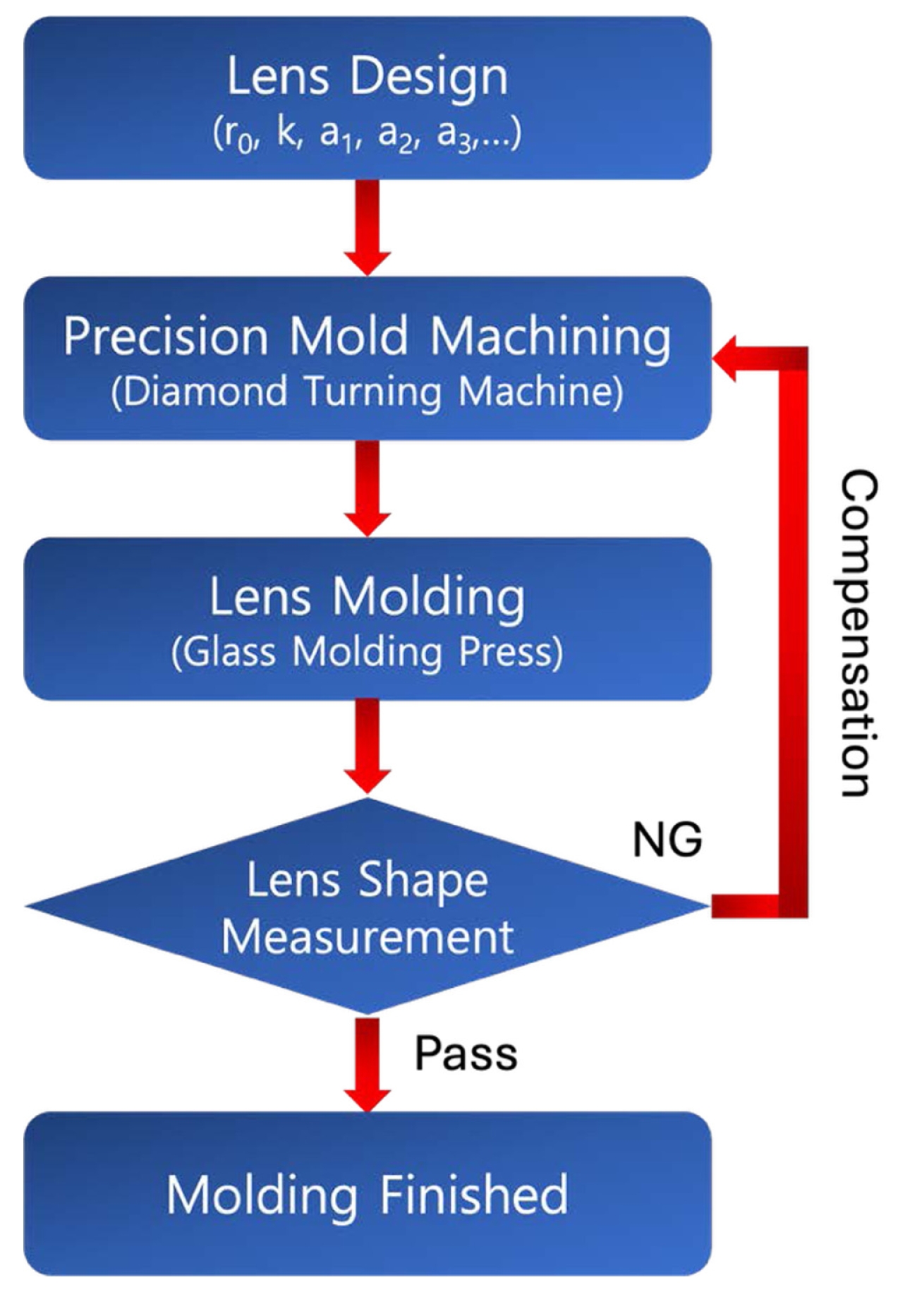
본 연구는 GMP 성형 비구면 유리 마이크로렌즈의 형상 측정 데이터를 활용하여, 파이썬으로 작성한 비구면 형상 보정 도구를 통해 열변형 오차를 보상하기 위한 최적화된 계수를 확보하고, 이를 통해 광통신 및 고출력 레이저 분야에서 요구되는 고정밀 결합 효율을 달성할 수 있는 금형 보정 설계 방법을 제시하는 것을 목적으로 한다(
Fig. 1).
2. 이론적 배경
2.1 비구면 방정식(Aspheric Equation)
본 연구에서 다루는 비구면 렌즈의 형상은 광학 설계 분야에서 가장 보편적으로 사용되는 표준 비구면 방정식으로 정의한다.
여기에서 r0는 비구면 렌즈의 곡률반경이고, k와 ai는 각각 코닉 상수(Conic constant)와 i차항에 대한 비구면 계수값을 나타낸다. 코닉상수에 따라 비구면 렌즈는 타원(Ellipse), 포물면(Parabola), 쌍곡선(Hyperbola) 로 나타낼 수 있다.
2.2 최소 제곱 피팅(Least-squares Fitting)
최소 제곱법은 측정 데이터에 가장 잘 맞는 곡선이나 함수를 찾는 표준 통계 방법으로, 잔차(Residual) 제곱의 합을 최소로 만드는 계수를 찾는 것이 목표이다. 잔차는 측정데이터와 설계 모델 간의 차이로
식(2)와 같다.
단순히 잔차의 합을 최소화하면 양수 오차와 음수 오차가 상쇄되어 잘못된 결과가 나올 수 있으므로, 모든 잔차를 양수로 만들기 위해 잔차를 제곱하여 더한다.
여기서 S(r0, k, ai)는 잔차 제곱의 합을 나타내며, 이 값이 최소가 되도록 r0, k, ai의 모든 변수를 찾는다.
3. 맞춤형 파이썬 피팅 도구 구현
3.1 도구의 아키텍처 및 모듈 구성
본 연구에서 개발한 파이썬 도구는 사용자 친화적인 GUI (Graphic User Interface)와 강력한 수치 해석 기능을 결합한 독립형 애플리케이션이다. 이 도구는
Table 1에서 소개하는 주요 파이썬 모듈과 구성요소로 이루어져 있다.
도구의 핵심 로직은 QWidget을 상속받는 MyApp 클래스 내에 구현되었다. 데이터 처리 과정은 다음과 같은 흐름을 따른다.
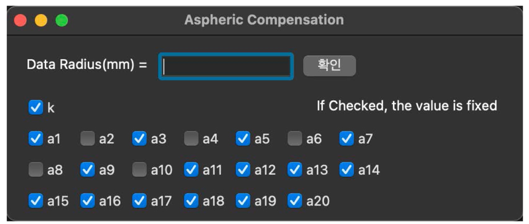
1) GUI 구성: 사용자는 비구면 형상을 보정하기 위한 영역을 지정하기 위해 렌즈 반경을 입력한다. 곡률반경(
r0)은 항상 변수로 설정하며, 코닉상수(k) 그리고 비구면 계수(
ai) 1차항부터 20차항까지의 21개의 파라미터에는 대응하는 체크 박스를 생성하여 피팅 시, 파라미터를 고정하거나 변수로 지정할 수 있도록 설정한다. 코드를 실행하면
Fig. 2와 같은 인터페이스가 나오게 된다.
2) 비구면 함수 정의: 20차항 표준 비구면 방정식을 아래와 같이 코닉상수에 따른
식(4)과 비구면 계수에 따른
식(5)으로 나눠 각각 정의하고, 이 함수를 lmfit의 피팅 모델로 사용한다.
3) 최소 제곱 피팅 실행: 렌즈의 설계 파라미터와 보정하고자 하는 렌즈의 측정데이터를 openpyxl을 이용하여 불러올 수 있도록 설정한다. lmfit.parameters()로 객체를 생성하고 로드된 초기 파라미터값을 할당한다. GUI의 체크박스 상태를 기반으로 각 계수에 대해 가변 또는 고정 속성을 부여한다. fmodel.fit() 명령을 실행하여 비선형 최소 제곱법을 통해 오차를 최소화하는 최적의 보정 계수를 산출한다. 이러한 논리를
Table 2와 같이 코드로 구성하였다.
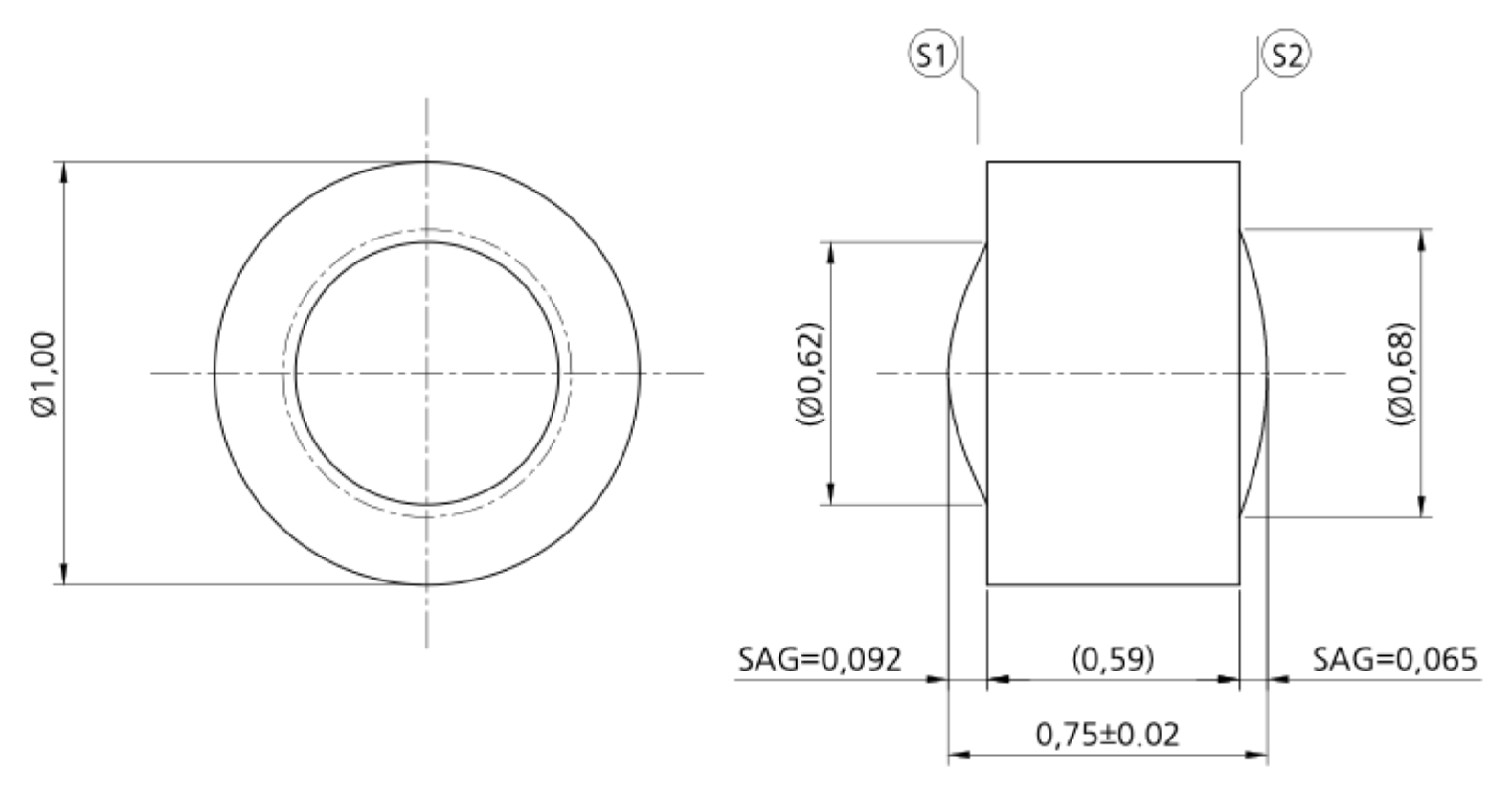
본 연구에서 개발한 파이썬 도구의 성능 검증을 위해 GMP 성형으로 제작한 비구면 유리 렌즈를 준비하였다. 양면이 볼록인 Bi-convex 형태의 렌즈로, 제1 광학 면(S1)은 곡률 반경과 코닉 상수로만 설계하였으며, 제2 광학 면(S2)은 곡률 반경과 코닉 상수에 더불어 4차항, 6차항 비구면 계수를 추가하여 설계하였다. 본 연구에서 사용한 렌즈의 설계 값은
Table 3과 같으며,
Fig. 3에서 렌즈의 개략도를 나타낸다.
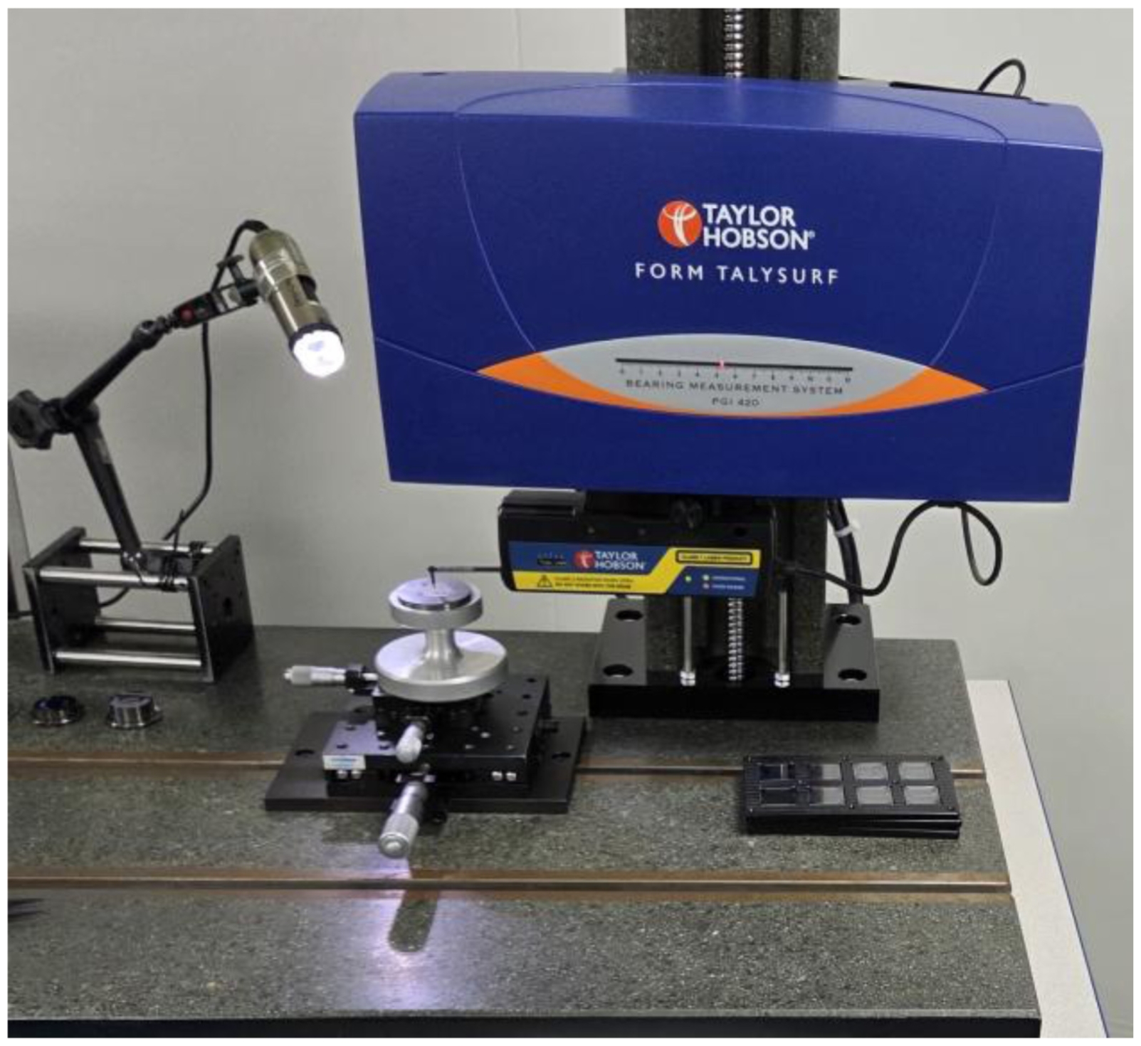
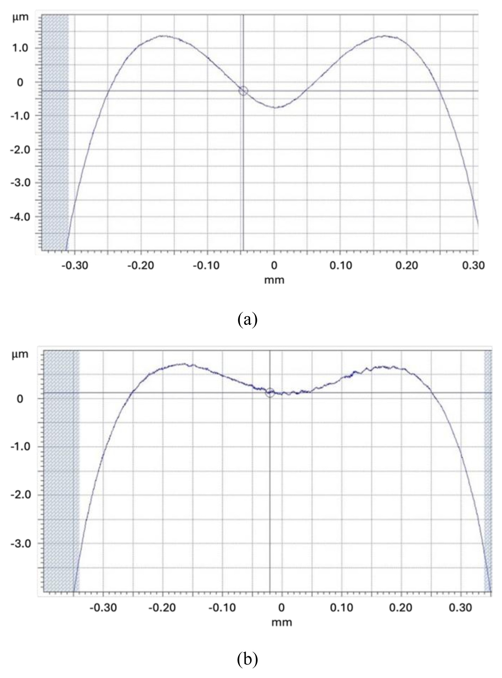
성형된 비구면 렌즈의 형상정도를 측정하기 위해 초정밀 접촉식 형상측정기(FORM TALYSURF PGI420; TAYLOR HOBSON, UK)를 사용하였다(
Fig. 4). 형상정도 (PV)는 각각 S1 5.93과 S2 4.02 μm으로 설계된 렌즈의 형상에서 크게 벗어남을 확인하였다(
Figs. 5(a) 및
5(b)).
비구면 렌즈의 측정한 실제 형상값과 설계값의 파라미터를
Tables 4 및
5에 나타내었으며, 열변형에 의해 파라미터가 서로 확연한 차이를 가짐을 알 수 있다.
4. 결과 분석
4.1 형상 보정 도구 결과창 구성
본 연구에서 개발한 형상 보정 도구를 실행 후 얻는 결과는
Table 6과 같이 보여준다. 크게 Fit Statistics, Variables, Correlations로 구성되어 있다.
Fit Statistics는 모델이 얼마나 잘 피팅되었는지 요약하여 통계적으로 보여주는 창으로, Fitting Method는 피팅을 수행하는 데 사용된 알고리즘을 의미하며 최소제곱법(Leastsq) 알고리즘을 사용했음을 알려준다. Function Evals은 최적화 과정에서 모델 함수를 평가(계산)한 횟수로, 50회 진행되었음을 시사한다. Data Point는 피팅에 사용된 데이터 포인트(N)의 총 개수를 의미하며, S1의 반경 0.32 mm를 0.01 mm 간격으로 총 33개 포인트로 구성된 측정데이터를 사용했다. Variables = 6은 피팅 과정 에서 그 값이 결정된 모델 파라미터의 개수(P)로, S1에서 코닉 상수는 고정시키고 보정 변수 파라미터로서 곡률반경, 2차, 4차, 6차, 8차, 10차항 비구면 계수를 변수로 지정하였다. Chi-square 는 카이제곱 통계량으로 잔차의 제곱합을 나타내며 이 값이 0에 가까울수록 모델이 데이터에 완벽하게 일치함을 의미한다. Reduced Chi-square는 자유도로 나눈 카이제곱 통계량으로, 여기서 자유도는 N-P(데이터 포인트 수-파라미터 수)이다. 이상적인 피팅일수록 이 값이 1에 가까워진다. R-squared는 결정 계수 로 모델이 데이터의 변동성을 얼마나 잘 설명하는지를 나타내 며 0에서 1 사이의 값을 가진다. 1의 값을 가진다는 것은 모델이 데이터의 모든 변동성을 완벽하게 설명한다는 의미로, 모델의 예측값과 실제 데이터가 일치한다는 것을 의미한다[
6].
Variables는 모델에 사용된 모든 매개변수의 최종 피팅 결과값을 보여준다. 구성은 매개변수: 최종피팅 값 표준오차(상대표준오차) (피팅의 초기 값)으로 나타내며, GUI 실행 창에서 가변으로 지정되지 않은 값들은 별도로(Fixed)로 표기된다.
Correlations는 피팅된 매개변수들 사이의 상호 의존성을 나타내는 상관 계수(Correlation Coefficient)를 보여준다. -1부터 1사이의 값을 가지며, 절대값이 0.100 미만인 약한 상관관계는 결과에 표기되지 않는다. 상관 계수가 +1에 가까우면 한 변수가 증가할경우, 다른 변수도 증가해야 잔차가 최소화되며, 반대로 -1에 가깝다면 한 변수가 증가할경우, 다른 변수는 감소해야 잔차가 최소화됨을 의미한다. 0에 가깝다면 두 변수는 서로에 거의 영향을 주지 않고 독립적이다.
4.2 성형 렌즈 형상 보정
형상 보정 도구를 이용하여 성형 렌즈의 S1, S2 면의 피팅을 진행하였다. 변수는 곡률 반경, 2차, 4차, 6차, 8차, 10차항 비구면 계수인 총 6개를 지정하였으며, 나머지는 설계값에 고정시켰다. 이에 따른 보정 파라미터는
Table 7처럼 얻었으며,
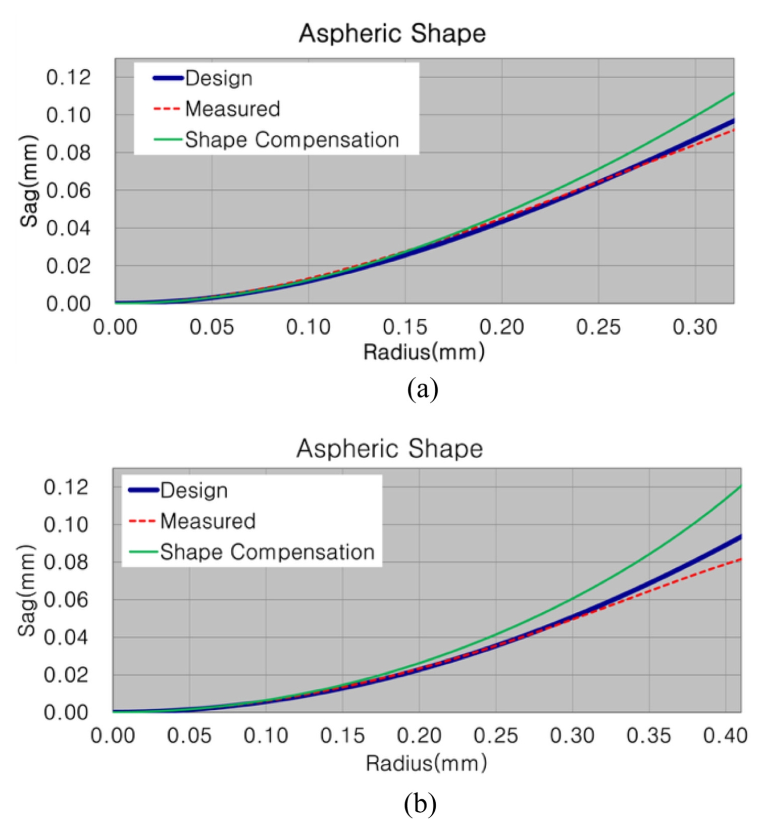
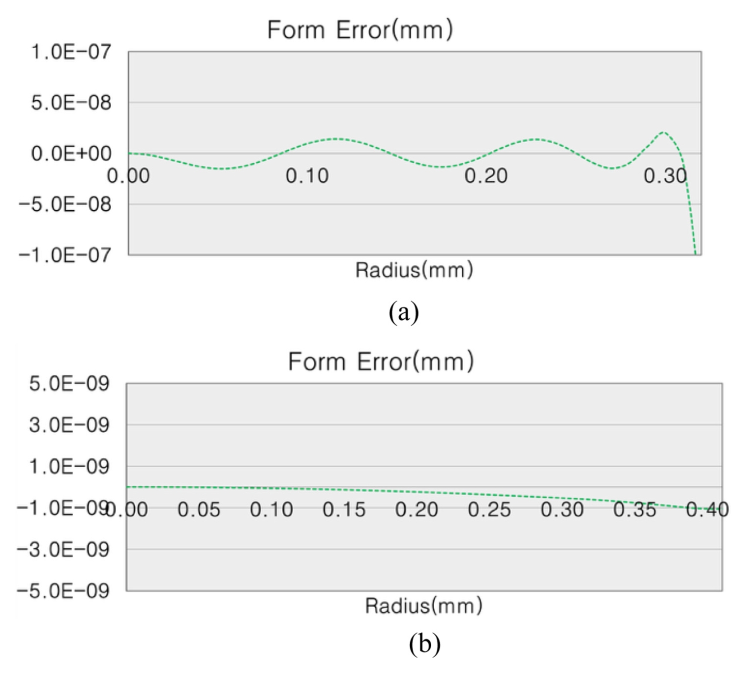
Fig. 6과 같이 설계 형상, 측정 형상 및 보정 형상을 비교하였다. 구상한대로 피팅이 잘 적용되었는지 확인하기 위해 설계 형상에 잔차를 더한 형상과 보정 형상 간의 형상오차(Form Error)를
Fig. 7처럼 나타내었다. S2 면은 ±1×10
-10 m 범위 내 형상 오차가 0에 수렴할만큼 좋은 결과를 얻었으나, S1 면은 불안정한 오차를 보여, 코닉상수를 변수로 추가 지정하여 7개 변수에 대한 형상 보정으로 다시 진행하였다.
S1 면에 대한 코닉상수를 변수에 추가하여 다시 보정 피팅한 파라미터는
Table 8과 같다.
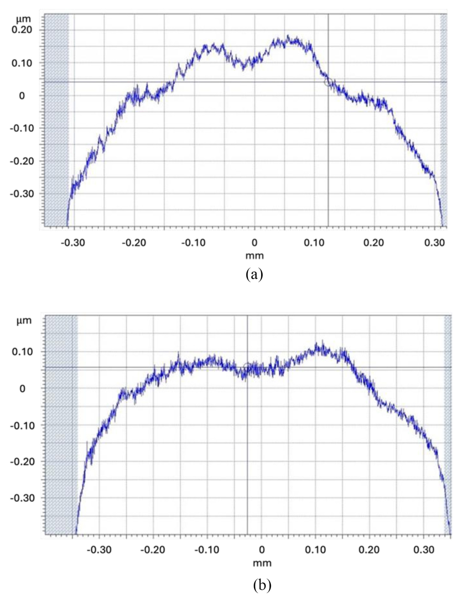
형상 보정 도구로 얻은 보정 파라미터를 이용하여 성형용 코어를 보정가공하고, 이 코어를 사용하여 비구면 유리 렌즈를 성형한 결과, 보정 전 성형 렌즈의 형상정도가 S1 5.93과 S2 4.02 μm에서 보정 후 형상정도가 S1 0.546과 S2 0.503 μm로 요구 사양에 만족할 수준으로 향상된 결과를 얻을 수 있었다(
Fig. 8).
2차항 비구면 계수는 기본 구면과 관련된 Conic Constant Term과 수학적으로 중첩된 항이며, 곡률과 강한 상관관계를 가진다. 이로 인해 렌즈의 근축(Paraxial) 성질에 영향을 주어 렌즈의 초점 거리(Focal Length), 배율(Magnification)이 바뀔 가능성이 있다. 광통신 또는 레이저 분야와 같은 비결상 광학계에서는 근축의 영향보다 높은 형상정밀도로 설계와 유사한 시스템 효율을 중시하므로 문제가 되지 않지만, 결상 광학계에서는 성능 저하로 이어질 수 있다. 따라서, 2차항을 보정 변수에서 제외하고 12차항, 14차항을 추가하여 보정을 진행하였으며,
Table 9와 같은 파라미터를 얻을 수 있다.
5. 결론
본 연구는 GMP 성형 비구면 유리 렌즈의 열변형 보상을 위해 비선형 최소 제곱 피팅을 이용한 비구면 계수 역추적 기법을 제안하고, 이를 사용자 정의 가능한 파이썬 GUI 코드로 구현하였다.
본 연구의 핵심 산출물인 맞춤형 파이썬 도구는 PyQt5, openpyxl, lmfit 등 모듈을 체계적으로 결합하여 개발되었으며, 사용자 정의 계수 가변성 제어라는 독창적인 기능을 제공한다.
이 도구의 유연성을 통해 GMP 열변형과 같은 복잡한 물리적 현상에 최적화된 피팅 모델을 구성할 수 있었으며, 이를 통해 산출된 보정 계수는 GMP 유리 렌즈의 형상 정밀도를 보정 전 약 4–5 μm에서 보정 후 약 0.5 μm으로 크게 향상시켜, 광통신 및 고출력 레이저 분야에서 요구되는 높은 광결합 효율을 달성하는 데 기여할 수 있을 것으로 기대한다. 또한, 근축에 영향을 주는 계수, 수차에 영향을 주는 계수 등의 22개의 매개변수를 사용자가 적절히 선택하여 보정 변수로 지정할 수 있으므로 결상 광학계에서도 유용한 도구로 기여할 수 있을 것으로 기대한다.
Fig. 1Schematic diagram of the aspheric lens molding system
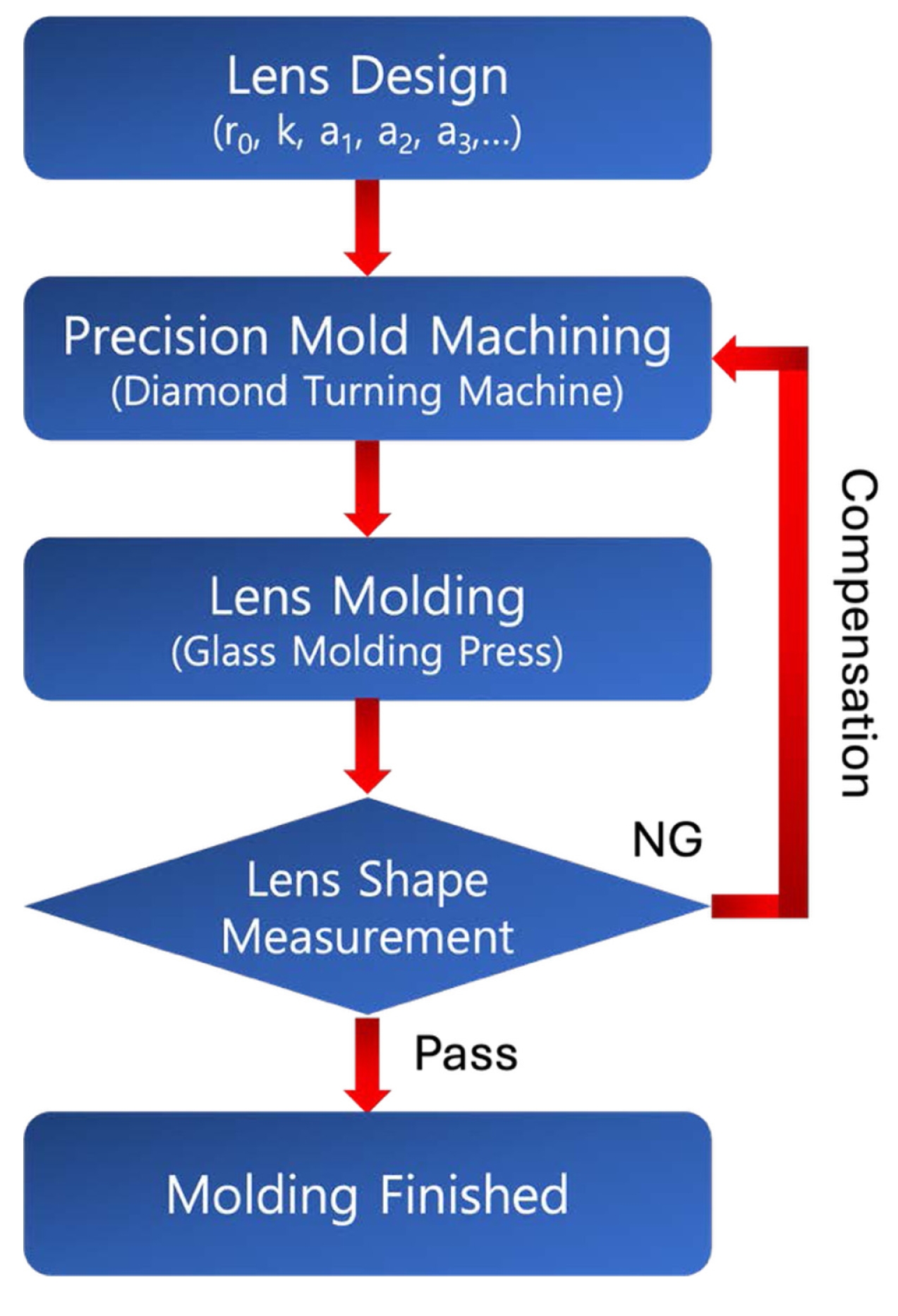
Fig. 2Configure the GUI (Graphic User Interface). Data radius sets the compensation area based on the measurement data. At the bottom of the interface, there are check marks to determine whether each parameter is variable or fixed during shape compensation
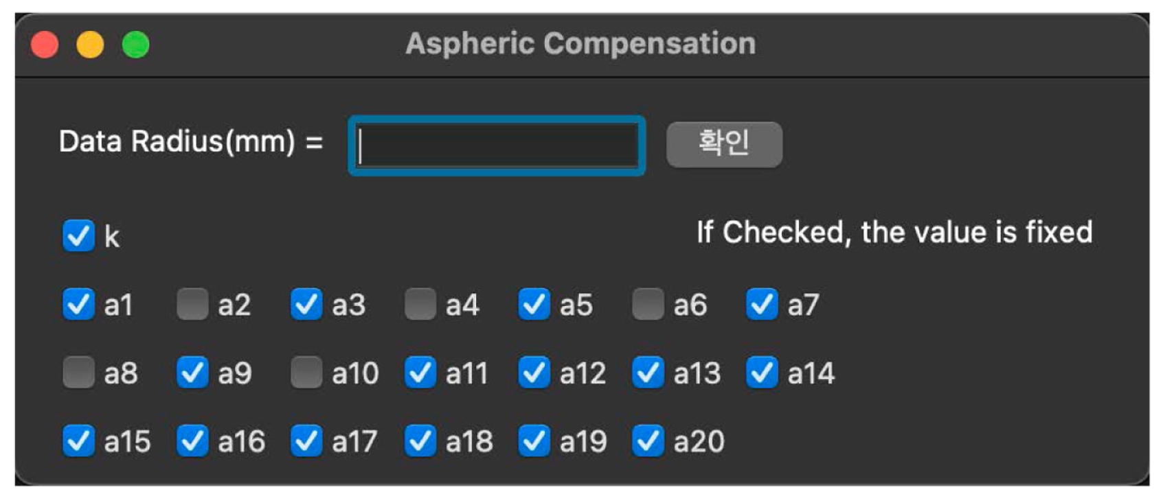
Fig. 3Schematic optical design of glass molded aspherical lens
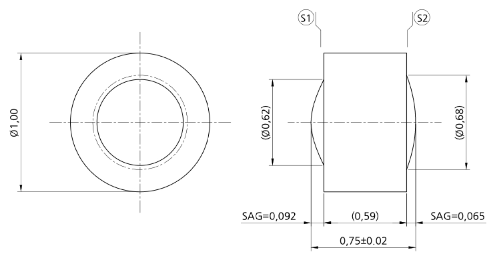
Fig. 4Aspherical lens shape measuring equipment: FTS PGI420
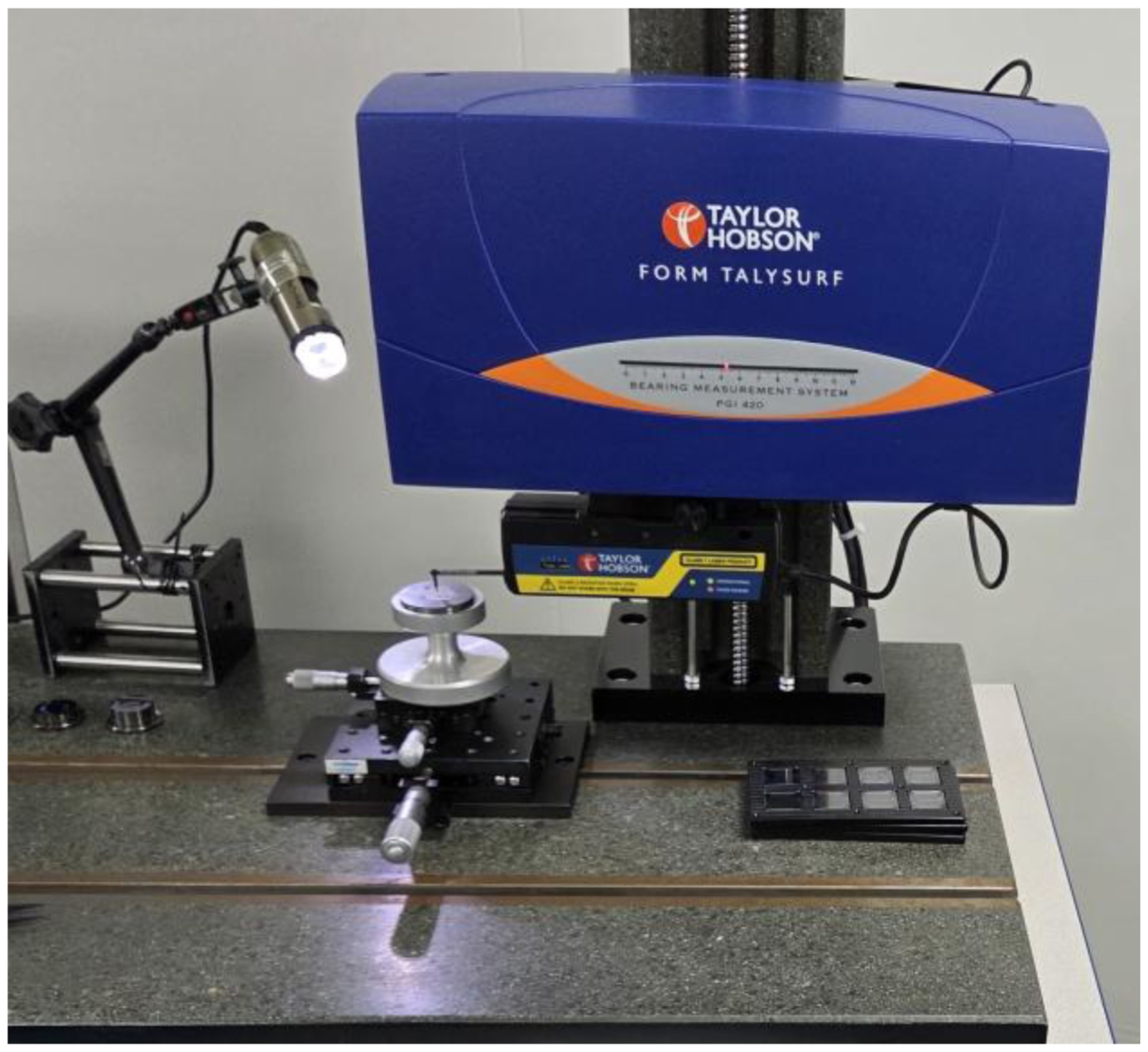
Fig. 5Lens form accuracy of (a) S1 surface (PV = 5.9327 μm) and (b) S2 surface (PV = 4.0294 μm)
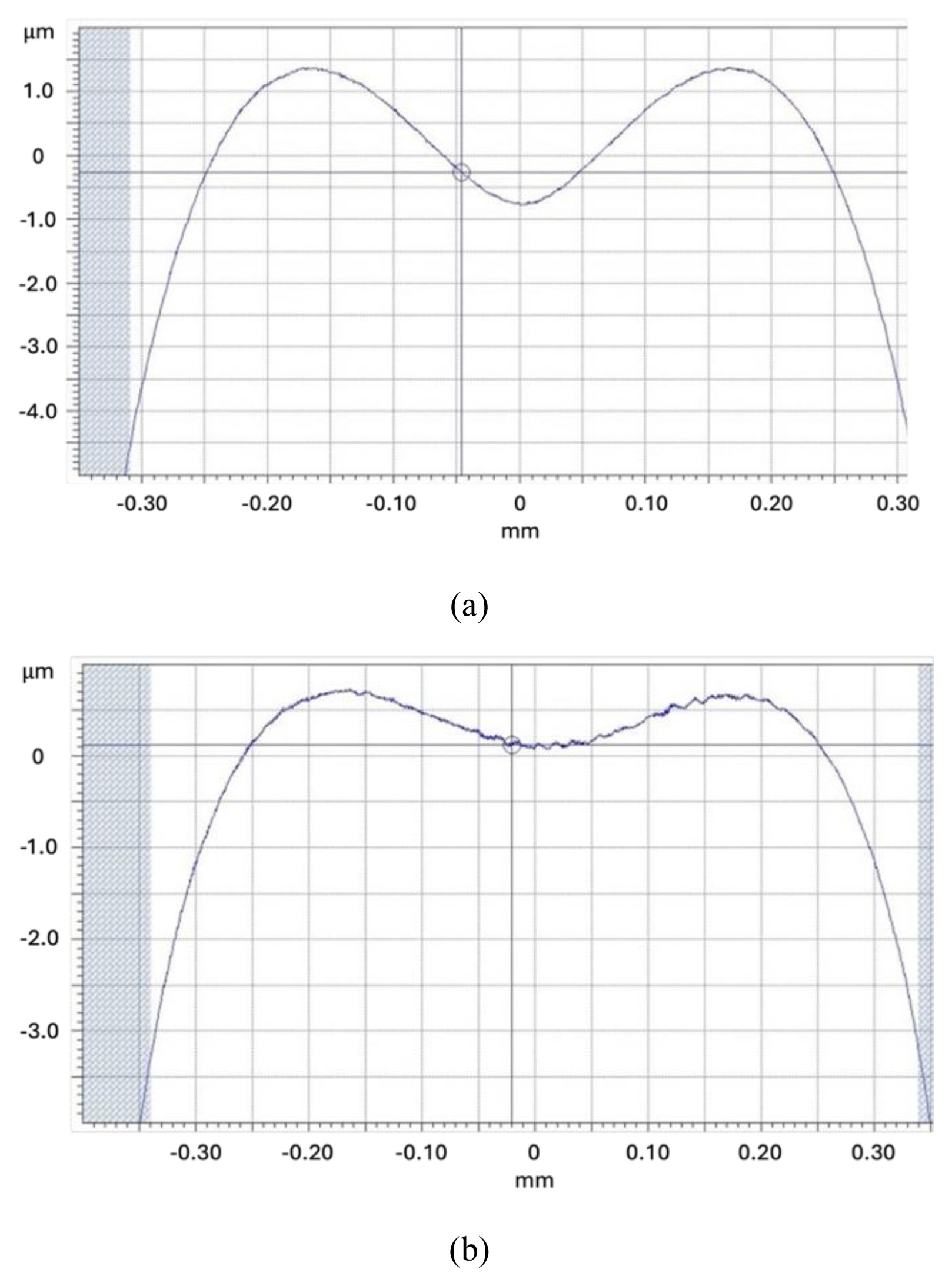
Fig. 6Comparison of aspheric shape (a) S1 surface and (b) S2 surface (Darkblue line: Design, Red dot: Measured and green line: Target shape compensation)
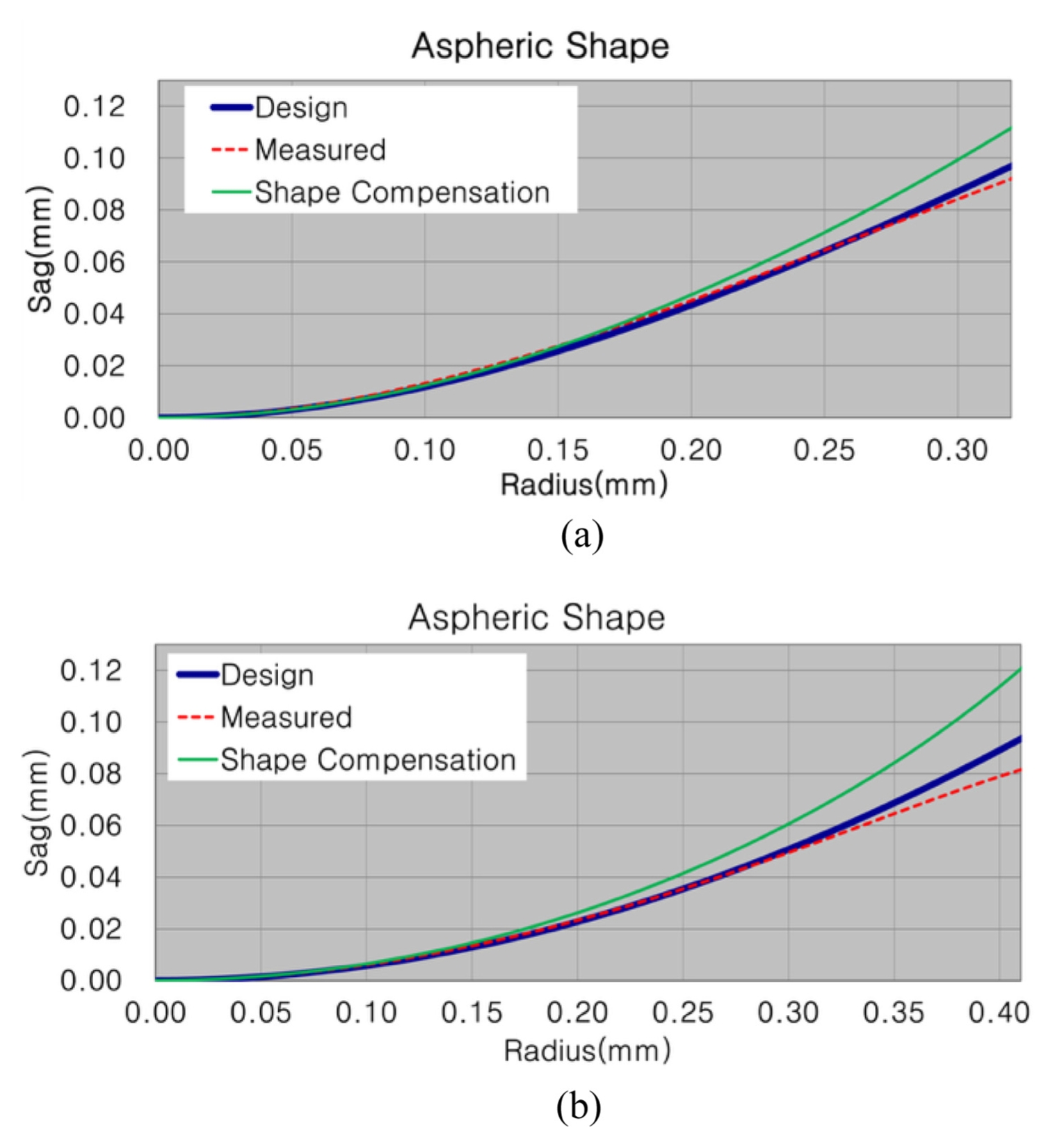
Fig. 7Form error graph for shape compensation: (a) S1 surface and (b) S2 surface
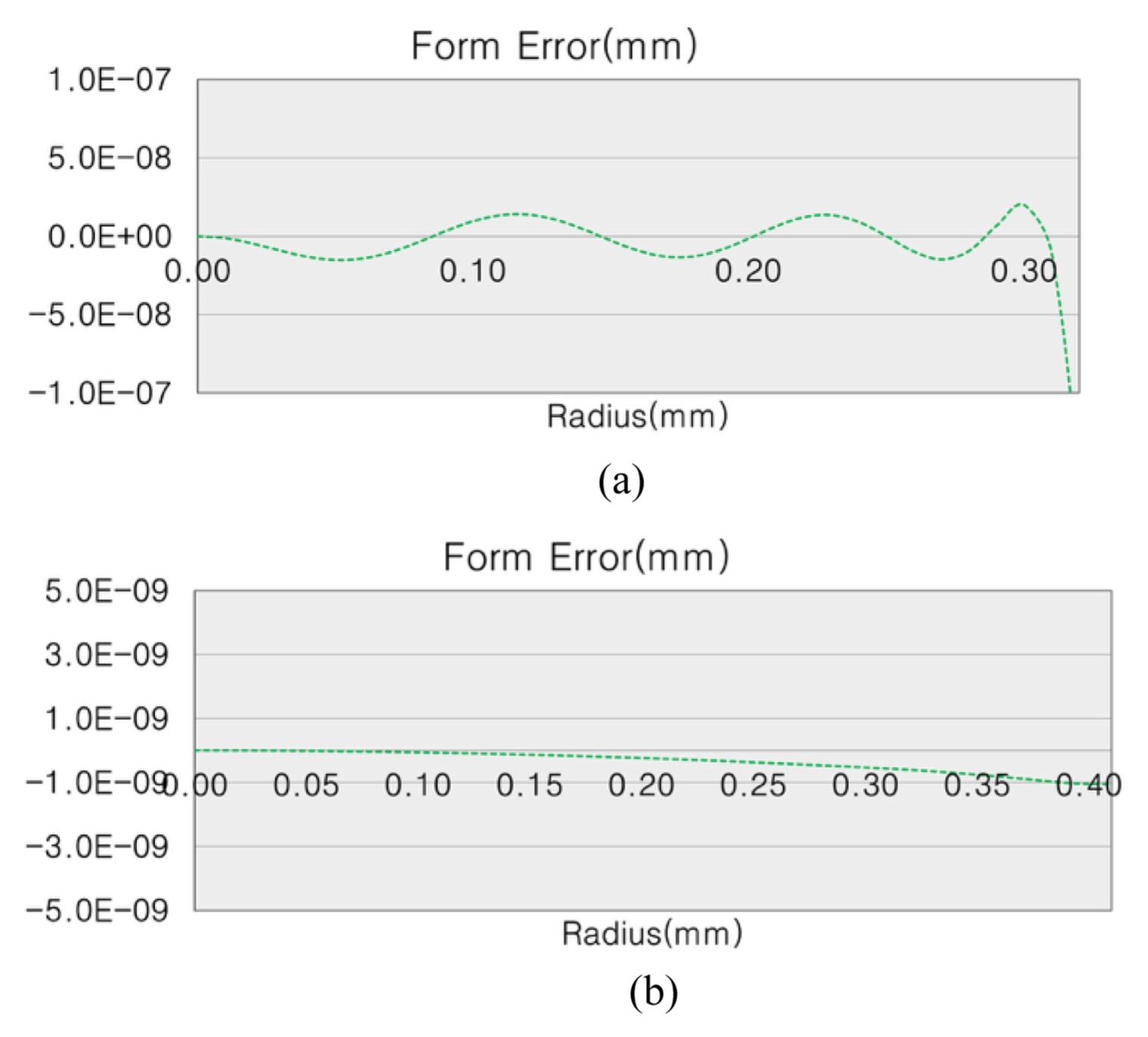
Fig. 8Lens form accuracy of (a) S1 surface (PV = 0.5464 μm) and (b) S2 surface (PV = 0.5030 μm)
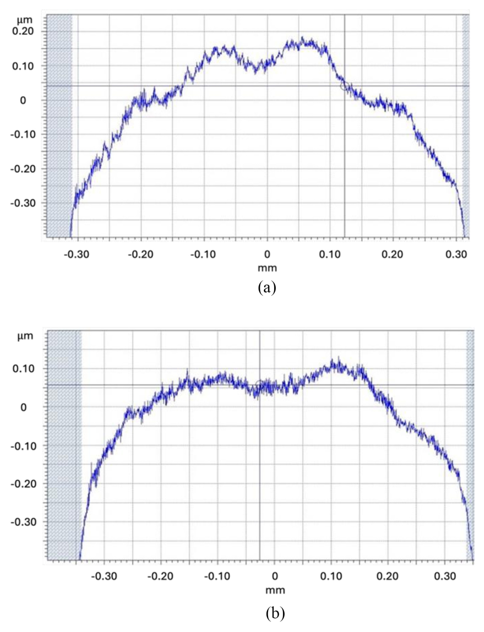
Table 1Python fitting tool: main components and modules
Table 1
|
Parameter |
Module |
Function |
|
GUI |
PyQt5 |
Providing a user interface for inputting data radius and controlling the variability of 20 aspheric coefficients and conic constant |
|
Core Calculation engine |
Lmfit [5], Numpy |
Nonlinear least-squares fitting of aspheric functions using lmfit and numpy |
|
Data I/O |
openpyxl, os, sys |
Load the measured raw data and initial coefficient values
Save the final compensation coefficient values to an excel file |
Table 2Python code: Logic for granting variable properties to lmfit’s parameter object
Table 2
|
fmodel = Model(asphere_complete) |
|
parameters = Parameters() |
|
r_max = np.max(x) |
|
parameters.add('r0', value=initial_values[0], vary=True) |
|
parameters.add('r_max', r_max, vary=False) |
|
parameters.add('k', value=initial_values[2], |
|
vary=parameters_vary['k']) |
|
for i in range(1, 21): |
|
parameters.add(f'a{i}', value=initial_values[i+2], |
|
vary=parameters_vary[f'a{i}']) |
|
result = fmodel.fit(z, parameters, x=x) |
|
print(result.fit_report()) |
Table 3Design parameter of glass molded aspherical lens
Table 3
|
Surface |
Radius [mm] |
Conic cons |
4th coef |
6th coef |
|
S1 |
4.063E-01 |
−3.533E+00 |
- |
- |
|
S2 |
8.700E-01 |
−1.634E+00 |
−7.845E-03 |
5.022E-02 |
Table 4Comparison of design and measured parameters on the surface of lens S1
Table 4
|
Parameter |
Design |
Measured |
|
Radius [mm] |
4.063E-01 |
4.217E-01 |
|
Conic constant |
−3.533E+00 |
−3.533E+00 |
|
2nd coef |
- |
2.419E-01 |
|
4th coef |
- |
−7.055E+00 |
|
6th coef |
- |
1.039E+02 |
|
8th coef |
- |
−8.983E+02 |
|
10th coef |
- |
2.996E+03 |
Table 5Comparison of design and measured parameters on the surface of lens S2
Table 5
|
Parameter |
Design |
Measured |
|
Radius [mm] |
8.700E-01 |
7.337E-01 |
|
Conic constant |
−1.634E+00 |
−1.634E+00 |
|
2nd coef |
- |
−4.705E-02 |
|
4th coef |
−7.845E-03 |
9.059E-01 |
|
6th coef |
5.022E-02 |
−6.052E+00 |
|
8th coef |
- |
3.675E+01 |
|
10th coef |
- |
−5.324E+01 |
Table 6Schematic diagram of the shape compensation tool results
Table 6
|
Fit statistics |
|
Fitting method |
leastsq |
|
Function evals |
50 |
|
Data points |
33 |
|
Variables |
6 |
|
Chi-square |
5.8506e-15 |
|
Reduced chi-square |
2.1669e-16 |
|
R-squared |
1.00000000 |
|
Variables |
Correlations |
|
Show the results for all parameters used in the model |
It shows the correlation coefficient, which indicates the interdependence between the fitted parameters |
Table 7Parameter results according to shape compensation on the S1 and S2 Lens surface
Table 7
|
Parameter |
S1 compensation |
S2 compensation |
|
Radius [mm]] |
3.412E-01 |
7.337E-01 |
|
Conic constant |
−3.533E+00 (fixed) |
−1.634E+00 (fixed) |
|
2nd coef |
−2.146E-01 |
−4.705E-02 |
|
4th coef |
6.836E+00 |
9.059E-01 |
|
6th coef |
−1.024E+02 |
−6.052E+00 |
|
8th coef |
8.914E+02 |
3.675E+01 |
|
10th coef |
−2.981E+03 |
−5.324E+01 |
Table 8Parameter results according to 2nd Shape compensation on the S1 lens surface
Table 8
|
Parameter |
S1 2nd compensation |
|
Radius [mm] |
3.148E-01 |
|
Conic constant |
−3.092E+00 |
|
2nd coef |
−3.375E-01 |
|
4th coef |
7.248E+00 |
|
6th coef |
−1.045E+02 |
|
8th coef |
8.999E+02 |
|
10th coef |
−2.998E+03 |
Table 9Parameter results according to 3rd shape compensation on the S1 and S2 lens surface
Table 9
|
Parameter |
S1 compensation |
S2 compensation |
|
Radius [mm] |
3.998E-01 |
7.881E-01 |
|
Conic constant |
−4.595E+00 |
−1.634E+00 |
|
2nd coef |
- |
- |
|
4th coef |
5.899E+00 |
8.671E-01 |
|
6th coef |
−9.507E+01 |
−6.017E+00 |
|
8th coef |
8.320E+02 |
3.671E+01 |
|
10th coef |
−2.607E+03 |
−5.321E+01 |
|
12th coef |
−1.477E+03 |
- |
|
14th coef |
2.624E+03 |
- |
REFERENCES
- 1. Lee, D., Kim, H., Cha, D., Lee, H., Kim, H., Kim, J., (2010), A Study on thermal deformation compensation in the molding of aspheric glass lenses, Journal of the Korean Society for Precision Engineering, 27(5), 22-26.
- 2. Kim, Y. C., (2006), A Study on measurement of aspheric lens and compensation of shrinkage on surfaces, M.Sc. Thesis, Graduate School of Industrial Technology and Management, Korea Polytechnic University.
- 3. Song, K., Kim, B., Yoon, H., Yang, J., Kim, K., Xiao, H., Cho, M., (2015), Aspherical lens design and injection mold analysis using extracted shape information, Transactions of Materials Processing, 24(6), 437-442.
- 4. Kim D.-I., Kim G.-H.. 2014;Reconstruction and method for unknown aspheric surface equations from measurement of aspheric surfaces. KR. 101425780B1.
- 5. Github, lmfit/lmfit.py. https://github.com/lmfit/lmfit-py.
- 6. Non-Linear Least-Squares Minimization and Curve-Fitting for Python, Performing fits and analyzing outputs. https://lmfit.github.io/lmfit-py/fitting.html#goodness-of-fit-statistics.
Biography
- Hyun Jong Kang
M.S. MPNICS Co., Ltd. His research interest includes fabrication and characterization of aspherical glass lens.
- Sang Do Kang
M.S. MPNICS Co., Ltd. His research interest includes fabrication and characterization of aspherical glass lens.
- Seung Keun Oh
Ph.D. MPNICS Co., Ltd. His research interest includes fabrication and characterization of aspherical glass lens.
- Woo Soon Kim
Professor in the Department of Mechanical Engineering, Wonkwang University. His research interest includes precision engineering.
Appendix